gmmEval

Evaluation of a GMM (Gaussian mixture model)

Contents

Syntax

Description

[logLike, gaussianProb] = gmmEval(data, gmmPrm) returns the log likelihood of a GMM model for each column of the given data matrix, where

data: dim x dataNum matrix where each column is a data point

gmmPrm(i): Parameters for Gaussian component i

• gmmPrm(i).mu: a mean vector of dim x 1
• gmmPrm(i).sigma: a covariance matrix of 3 possible dimensions:
  • 1 x 1: identity covariance matrix times a constant for each Gaussian
  • dim x 1: diagonal covariance matrix for each Gaussian
  • dim x dim: full covariance matrix for each Gaussian
• gmmPrm(i).w: a weighting factor

chunkSize: size of a chunk for vectorization

• 1 for fully for-loop version
• inf for fully vectorized version (which could cause "out of memory" is data size is large)
• (To see the effects of chunkSize, try gmmEvalSpeedTest.m under test folder of DCPR toolbox.)

logLike: 1 x dataNum vector of output probabilities

gaussianProb(i,j) is the probability of data(:,j) to the i-th Gaussian (This is for gmmTrain.m only)

Example

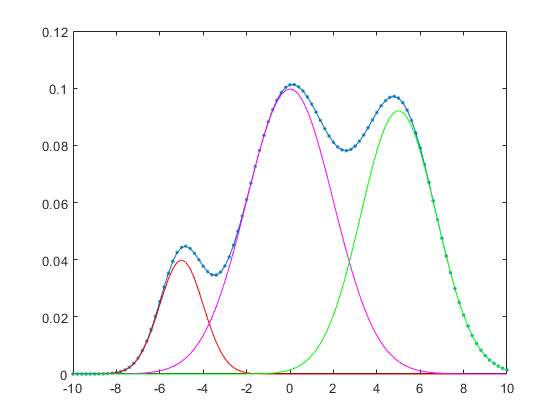
The following example plots GMM results of 1-D data:

data=linspace(-10, 10, 101);
gmmPrm(1).mu = -5; gmmPrm(1).sigma = 1; gmmPrm(1).w = 0.1;
gmmPrm(2).mu =  0; gmmPrm(2).sigma = 4; gmmPrm(2).w = 0.5;
gmmPrm(3).mu =  5; gmmPrm(3).sigma = 3; gmmPrm(3).w = 0.4;
logLike = gmmEval(data, gmmPrm);
prob=exp(logLike);
figure; plot(data, prob, '.-');
line(data, gmmPrm(1).w*gaussian(data, gmmPrm(1)), 'color', 'r');
line(data, gmmPrm(2).w*gaussian(data, gmmPrm(2)), 'color', 'm');
line(data, gmmPrm(3).w*gaussian(data, gmmPrm(3)), 'color', 'g');

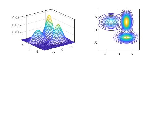
The following example plots GMM results of 2-D data:

gmmPrm(1).mu = [-3, 3]'; gmmPrm(1).sigma = [5, 2]'; gmmPrm(1).w = 0.3;
gmmPrm(2).mu = [3, -3]'; gmmPrm(2).sigma = [4, 1]'; gmmPrm(2).w = 0.3;
gmmPrm(3).mu =  [3, 3]'; gmmPrm(3).sigma = [1, 4]'; gmmPrm(3).w = 0.4;
bound = 8;
pointNum = 51;
x = linspace(-bound, bound, pointNum);
y = linspace(-bound, bound, pointNum);
[xx, yy] = meshgrid(x, y);
data = [xx(:), yy(:)]';
logLike = gmmEval(data, gmmPrm);
zz = reshape(exp(logLike), pointNum, pointNum);
subplot(2,2,1);
mesh(xx, yy, zz); axis tight; box on
subplot(2,2,2);
contour(xx, yy, zz, 30); axis image; box on

See Also

gmmTrain.

Published with MATLAB® R2018a