[chinese][all]

Slides: DTW, DTW for melody recognition, DTW for speech recognition

The distance between two point $\mathbf{x}=[x_1, x_2, ..., x_n]$ and $\mathbf{y}=[y_1, y_2, ..., y_n]$ in a n-dimensional space can be computed via the Euclidean distance: $$ dist(\mathbf{x},\mathbf{y})=\|\mathbf{x}-\mathbf{y}\|=\sqrt{(x_1-y_1)^2+(x_2-y_2)^2+\cdots+(x_n-y_n)^2}. $$

However, if the length of $\mathbf{x}$ is different from $\mathbf{y}$, then we cannot use the above formula to compute the distance. Instead, we need a more flexible method that can find the best mapping from elements in $\mathbf{x}$ to those in $\mathbf{y}$ in order to compute the distance.

The goal of dynamic time warping (DTW for short) is to find the best mapping with the minimum distance by the use of DP. The method is called "time warping" since both $\mathbf{x}$ and $\mathbf{y}$ are usually vectors of time series and we need to compress or expand in time in order to find the best mapping. We shall give the formula for DTW in this section.

Let $\mathbf{t}$ and $\mathbf{r}$ be two vectors of lengths $m$ and $n$, respectively. The goal of DTW is to find a mapping path $\{(p_1, q_1), (p_2, q_2), ..., (p_k, q_k)\}$ such that the distance on this mapping path $\sum_{i=1}^k |t(p_i)-r(q_i)|$ is minimized, with the following constraints:

• Boundary conditions: $(p_1, q_1)=(1,1)$, $(p_k, q_k)=(m,n)$. This is a typical example of "anchored beginning" and "anchored end".
• Local constraint: For any given node $(i, j)$ in the path, the possible fan-in nodes are restricted to $(i-1, j)$, $(i, j-1)$, $(i-1, j-1)$. This local constraint guarantees that the mapping path is monotonically non-decreasing in its first and second arguments. Moreover, for any given element in $\mathbf{t}$, we should be able to find at least one corresponding element in $\mathbf{r}$, and vice versa.

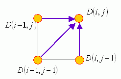
How can we find the optimum mapping path in DTW? An obvious choice is forward DP, which can be summarized in the following three steps:

1. Optimum-value function: Define $D(i, j)$ as the DTW distance between $t(1:i)$ and $r(1:j)$, with the mapping path starting from $(1, 1)$ to $(i, j)$.
2. Recursion: $$ D(i, j)=|t(i) - r(j)| + min \left\{\begin{matrix} D(i-1, j)\\D(i-1, j-1)\\D(i, j-1) \end{matrix}\right\}, $$ with the initial condition $D(1, 1)=|t(1)-r(1)|$.
3. Final answer: $D(m, n)$.

In practice, we need to construct a matrix D of dimensions m×n first and fill in the value of $D(1, 1)$ by using the initial condition. Then by using the recursive formula, we fill the whole matrix one element at a time, by following a column-by-column or row-by-row order. The final answer will be available as $D(m, n)$, with a computational complexity of $O(mn)$.

If we want to know the optimum mapping path in addition to the minimum distance, we may want to keep the optimum fan-in of each node. Then at the end of DP, we can quickly back track to find the optimum mapping path between the two input vectors.

We can also have the backward DP for DTW, as follows:

1. Optimum-value function: Define $D(i, j)$ as the DTW distance between $t(i:m)$ and $r(j:n)$, with the mapping path from $(i, j)$ to $(m, n)$.
2. Recursion: $$ D(i, j) = |t(i) - r(j)| + min\left\{\begin{matrix}D(i+1, j)\\D(i+1, j+1)\\D(i, j+1)\end{matrix}\right\},$$ with the initial condition $D(m, n) =|t(m) - r(n)|$.
3. Final answer: $D(1, 1)$.

The answer obtain by the backward DP should be that same as that obtained by the forward DP.

Another commonly used local path constraint is to set the fan-in of 27°-45°-63° only, as shown in the following figure:

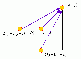
The use of this local path constraint leads to the following potential results:

• Some points in the input vectors could be skipped in the mapping path. This is advantageous if the input vectors contains sporadic outliners.
• Since the optimum-value function is based on the total distance, sometimes the mapping path will take the local paths of 27° or 63° instead of 45° in attempting to minimize the total distance.

If the required mapping path is "anchored beginning, anchored end", then the local path constraints can induce the global path constraints, as shown next:

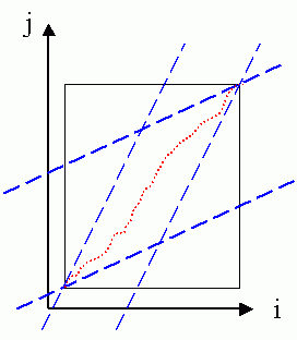
In the above figure, the feasible region for the mapping path is shown as a parallelogram. In filling up the matrix, we can save computation by skipping the elements outside the parallelogram. In addition, a feasible mapping exists only when the ratio of the input vectors' lengths are between 0.5 and 2.

If the required mapping path is "anchored beginning and free end" (which is used for query by singing or humming), then the induced global path constraints are shown next:

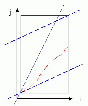
The feasible region for the mapping path is shown as a trapezoid in the above figure. Compared with the case of "anchored beginning and anchored end", we can save less computation by using this set constraints.

If the required mapping path is "free beginning and free end" (which is used for speaker-dependent keyword spotting), then the induced global path constraints are shown next:

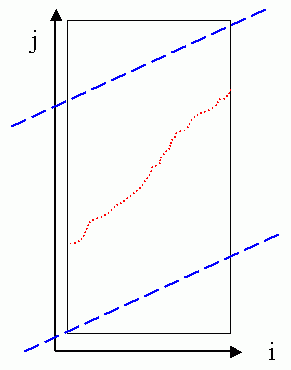
The feasible region for the mapping path is shown as a parallelogram in the above figure. Compared with the case of "anchored beginning and free end", we can save less computation by using this set constraints.

It should be noted that the global path constraints are induced as a result of the local path constraints of 27°-45°-63°. However, when we are using the local path constraints of 0°-45°-90°，sometimes we still apply the global path constraints in order to limit the mapping path to a reasonable shape. In summary, the use of global path constraints serves two purposes:

• Reduce computation load.
• Limit the mapping path to be a reasonable one.

In the following, we shall give some examples of DTW. For simplicity, we shall distinguish two types of DTW:

• Type-1 DTW uses 27°-45°-63° local path constraint.
• Type-2 DTW uses 0°-45°-90° local path constraint.

First, we can use dtw.m (with dtwOpt.type=1) and dtwPathPlot.m to plot the mapping path of type-1 DTW in the following example:

Example 1: dtw1Plot01.m

vec1=[71 73 75 80 80 80 78 76 75 73 71 71 71 73 75 76 76 68 76 76 75 73 71 70 70 69 68 68 72 74 78 79 80 80 78]; vec2=[69 69 73 75 79 80 79 78 76 73 72 71 70 70 69 69 69 71 73 75 76 76 76 76 76 75 73 71 70 70 71 73 75 80 80 80 78]; dtwOpt=dtwOptSet; dtwOpt.type=1; [minDist, dtwPath, dtwTable] = dtw(vec1, vec2, dtwOpt); dtwPathPlot(vec1, vec2, dtwPath);

In the above example, we deliberately put an outliner in vec1. Due to the local path constraints of type-1 DTW, this outliner is skipped in the optimum mapping path.

Similarly, we can use dtw.m (with dtwOpt.type=2) and dtwPathPlot.m to plot the mapping path of type-2 DTW:

Example 2: dtw2Plot01.m

vec1=[71 73 75 80 80 80 78 76 75 73 71 71 71 73 75 76 76 68 76 76 75 73 71 70 70 69 68 68 72 74 78 79 80 80 78]; vec2=[69 69 73 75 79 80 79 78 76 73 72 71 70 70 69 69 69 71 73 75 76 76 76 76 76 75 73 71 70 70 71 73 75 80 80 80 78]; dtwOpt=dtwOptSet; dtwOpt.type=2; [minDist, dtwPath, dtwTable] = dtw(vec1, vec2, dtwOpt); dtwPathPlot(vec1, vec2, dtwPath);

The outliner cannot be skipped since the local path constraints require each point in a vector has at least one correspondence in the other vector.

By using dtwBridgePlot.m, we can use red lines to connect corresponding points in two vectors, as follows:

Example 3: dtwBridgePlot02.m

vec1=[71 73 75 80 80 80 78 76 75 73 71 71 71 73 75 76 76 68 76 76 75 73 71 70 70 69 68 68 72 74 78 79 80 80 78]; vec2=[69 69 73 75 79 80 79 78 76 73 72 71 70 70 69 69 69 71 73 75 76 76 76 76 76 75 73 71 70 70 71 73 75 80 80 80 78]; dtwOpt=dtwOptSet; dtwOpt.type=1; [minDist1, dtwPath1, dtwTable1] = dtw(vec1, vec2, dtwOpt); dtwOpt.type=2; [minDist2, dtwPath2, dtwTable2] = dtw(vec1, vec2, dtwOpt); subplot(2,1,1); dtwBridgePlot(vec1, vec2, dtwPath1); title('DTW alignment by type-1 DTW'); subplot(2,1,2); dtwBridgePlot(vec1, vec2, dtwPath2); title('DTW alignment by type-2 DTW');

It becomes more obvious that type-1 DTW can have empty correspondence while type-2 DTW can have multiple correspondences. Moreover, we can use an extra argument for dtwBridgePlot.m to put the two vectors in 3D space to have a more interesting representation:

Example 4: dtwBridgePlot03.m

vec1=[71 73 75 80 80 80 78 76 75 73 71 71 71 73 75 76 76 68 76 76 75 73 71 70 70 69 68 68 72 74 78 79 80 80 78]; vec2=[69 69 73 75 79 80 79 78 76 73 72 71 70 70 69 69 69 71 73 75 76 76 76 76 76 75 73 71 70 70 71 73 75 80 80 80 78]; dtwOpt=dtwOptSet; dtwOpt.type=1; [minDist1, dtwPath1, dtwTable1] = dtw(vec1, vec2, dtwOpt); dtwOpt.type=2; [minDist2, dtwPath2, dtwTable2] = dtw(vec1, vec2, dtwOpt); subplot(2,1,1); dtwBridgePlot(vec1, vec2, dtwPath1, '3d'); title('DTW alignment by type-1 DTW'); view(-10, 70); subplot(2,1,2); dtwBridgePlot(vec1, vec2, dtwPath2, '3d'); title('DTW alignment by type-2 DTW'); view(-10, 70);

---

Data Clustering and Pattern Recognition (資料分群與樣式辨認)