(請注意:中文版本並未隨英文版本同步更新!)
Slides
Dynamic programming (DP) is an effective method for finding an optimum solution to a multi-stage decision problem, as long as the solution can be defined recursively. DP roots in the principle of optimality proposed by Richard Bellman:
「動態規劃」(Dynamic Programming,簡稱 DP)是一個很有效的方法來求得一個問題的最佳解,DP 的精神是來自於 Richard Bellman 所提出的 Principle of Optimality:
An optimal policy has the property that whatever the initial state and the initial decisions are, the remaining decisions must constitute an optimal policy with regard to the state resulting from the first decision.
In terms of path finding problems, the principle of optimality states that any partial path of the optimum path is also an optimum path given the starting and ending nodes. This is an obvious principle that can be proved by contradiction. In practice, a number of seemingly unrelated applications can be effectively solved by DP.
簡單地說,就是在一條最佳路徑上,其中任一條子路徑(Partial Path)也都必須是相關子問題的最佳路徑,否則原路徑就不是最佳路徑。這是一個很明顯的道理,可以很直覺地使用矛盾法來加以證明,可是在實際應用上面,可以有許多複雜的變形。
To employ the procedure of DP to solve a problem, usually we need to specify the following items:
- Define the optimum-value function.
- Derive the recursive formula for the optimum-value function, together with its initial condition.
- Specify the answer of the problem in term of the optimum-value function.
We shall give an example of DP for a path finding problem shown in the following graph:
舉例來說,以下列的圖形為例:
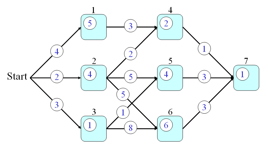
In the above graph, we assume that:
- Every node is a city and we use q(a) to represent the time required to go through node a, where a is in {1, 2, 3, 4, 5, 6, 7}.
- Every link is a route connecting two city. We use p(a, b) to represent the time required to go from nodes a to b, where a and b are in {1, 2, 3, 4, 5, 6, 7}.
假設:
- 每一條連結(Link)代表一條公路,連結上的數字則代表通過此公路所需的時間。我們使用 p(a, b) 來代表通過連接 Node a 和 Node b 的公路所需的時間。
- 每一個節點(Node)代表一個城市,節點上的數字則代表通過此程式所需的時間。我們使用 q(a) 來代表通過 Node a 所需的時間。
From the start point, how can we find a path that requires the minimum time to pass through node 7? This is a typical problem of DP which can be solved systematically and efficiently by the following three steps:
假設起點是 Start,終點是 Node 7,請問我們如何找到一條路徑,使得從起點到終點所花的時間最短?這是一個很典型的 DP 問題,我們可以經由下列三個步驟來迅速地解決這個問題:
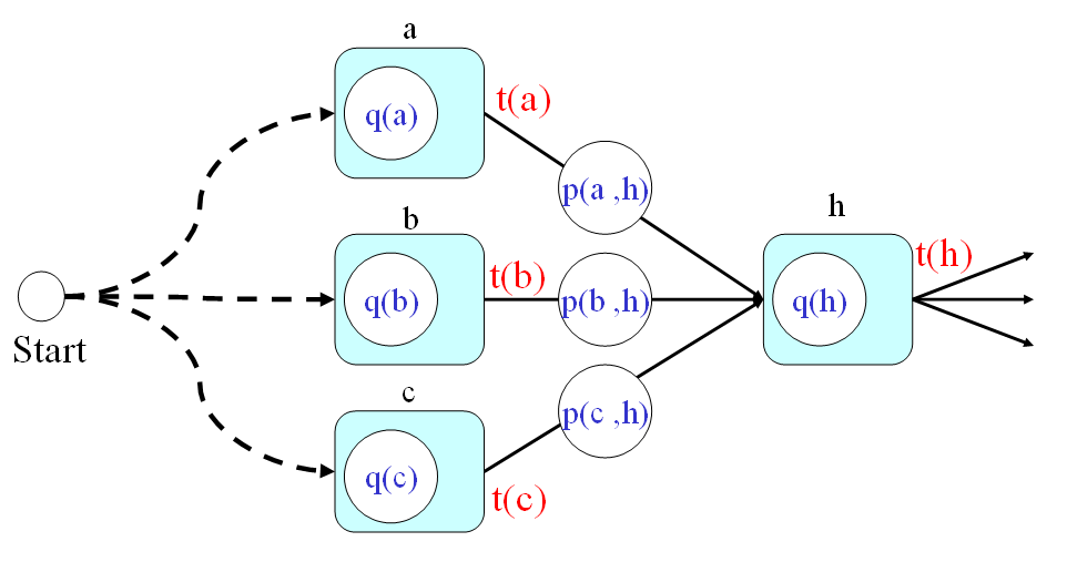
- First of all, we can define the optimum-value function t(h) as the minimum time from the start point to node h (including the time for passing node h).
- Secondly, the optimum-value function should satisfy the following recursive formula:
t(h) = min{t(a)+p(a,h), t(b)+p(b,h), t(c)+p(c,h)} + q(h) In the above equation, we assume the fan-ins of node h are a, b, and c. Please refer to the next figure.
在上述方程式中,我們假設連接到 Node h 的節點有三個,分別是 a, b, c。示意圖如下:
- And finally, the answer to the original problem should be t(7). By using the recursion, we can have the following steps for computing the time required by the optimum path:
- t(0) = 0
- t(1) = t(0)+4+5 = 9
- t(2) = t(0)+2+4 = 6
- t(3) = t(0)+3+1 = 4
- t(4) = min(9+3, 6+2)+2 = 10
- t(5) = min(6+5, 4+1)+4 = 9
- t(6) = min(6+5, 4+8)+6 = 17
- t(7) = min(10+1, 9+3, 17+3)+1 = 12
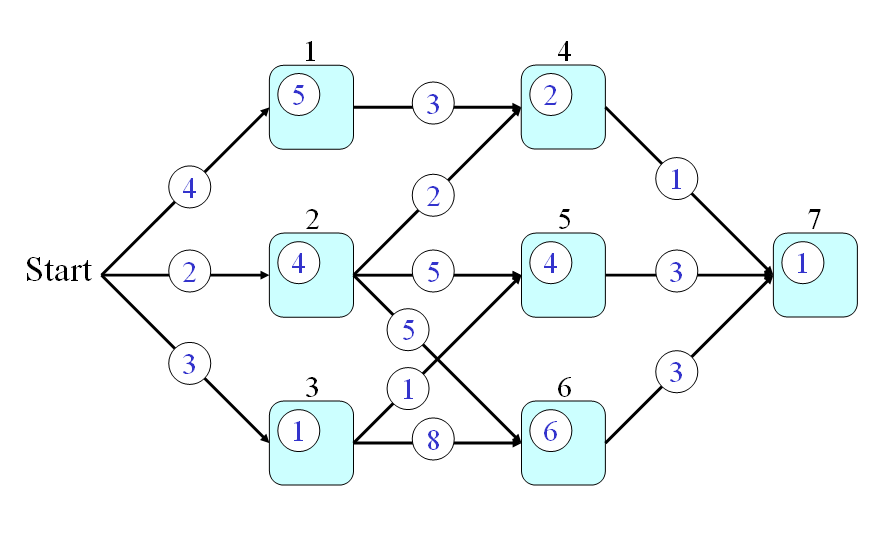
- Firstly, the optimum-value function s(h) is defined as the minimum time from a node h to the end node (including the time for passing the end node but excluding the time for passing node h.)
- Secondly, the optimum-value function should satisfy the following recursive formula:
s(h) = q(h) + min{p(h,a)+s(a), p(h,b)+s(b), p(h,c)+s(c)} where a, b, c are the fan-out of node h. The initial condition is s(7) = q(7). - Finally, the answer to the original problem is s(0). By using the recursion, we can have the following steps for computing the time required by the optimum path:
- s(7) = 1
- s(6) = q(6)+3+s(7) = 6+3+1 = 10
- s(5) = q(5)+3+s(7) = 4+3+1 = 8
- s(4) = q(4)+1+s(7) = 2+1+1 = 4
- s(3) = q(3)+min{1+s(5), 8+s(6)} = 1 + min{9, 18} = 10
- s(2) = q(2)+min{2+s(4), 5+s(5), 5+s(6)} = 4 + min{6, 13, 15} = 10
- s(1) = q(1)+3+s(4) = 5 + 3 + 4 = 12
- s(0) = min{4+s(1), 2+s(2), 3+s(3)} = min(16, 12, 13} = 12
The efficiency of DP is based on the fact that we can use some previous results iteratively. Some common characteristics of DP are summarized as follows:
- After finding the optimum fan-in path of a given node, it would be better to keep this information in the data structure in order to back track the optimum path at the end of DP.
- DP usually only gives the optimum path. If we want to find the second-best path, we need to invoke another version of DP to find the n-best path, which is beyond the scope of this tutorial.
換句話說,在我們計算 DP 的過程中,可以反覆利用先前所計算出來的結果,而省掉許多不必要的運算。DP 的特性,可列出如下:
- 在計算 DP 的過程中,必須在每個節點記錄最佳路徑的來源,才能在走到終點後,經由回溯(Back Tracking)來找到整個過程的最佳路徑。
- 若要尋求第二最佳路徑,則必須使用較複雜的 Top-N 計算方法,而不能只靠上述簡單的 DP 算法。
Data Clustering and Pattern Recognition (資料分群與樣式辨認)
