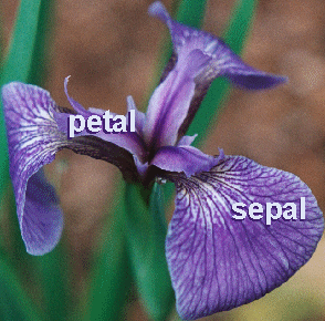
Iris dataset is by far the earliest and the most commonly used dataset in the literature of pattern recognition. The dataset contains 150 instances of iris flowers collected in Hawaii. These instances are divided into 3 classes of Iris Setosa, Iris Versicolour and Iris Virginica, based on 4 measures of sepal's width and length, and petal's width and length. These measures are taken for each iris flower, as shown next:

| 
| 
|
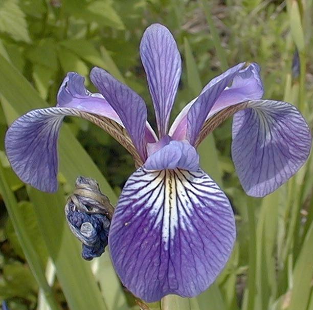
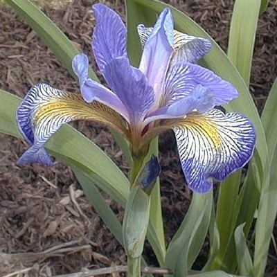
| Iris Setosa (More info) | Iris Versicolor (More info) | Iris Virginica (More info) |
- 4 features with numerical values, with no missing data
- sepal length in cm
- sepal width in cm
- petal length in cm
- petal width in cm
- 3 classes, including Iris Setosa, Iris Versicolour, Iris Virginica
- data size: 150 entries
- data distribution: 50 entries for each class
Iris 資料集可說是在樣式辨認研究中,最常被引用到的資料集,此資料集包含鳶尾花的資料,的特性如下:
- 特徵:共四種,都是數值,沒有未知量:
- sepal length in cm
- sepal width in cm
- petal length in cm
- petal width in cm
- 類別:共三類,包含 Iris Setosa, Iris Versicolour, Iris Virginica
- 資料筆數:150筆
- 類別分佈:各50筆
- Fisher,R.A. "The use of multiple measurements in taxonomic problems" Annual Eugenics, 7, Part II, 179-188 (1936); also in "Contributions to Mathematical Statistics" (John Wiley, NY, 1950).
- Duda,R.O., & Hart,P.E. (1973) Pattern Classification and Scene Analysis. (Q327.D83) John Wiley & Sons. ISBN 0-471-22361-1. See page 218.
- Dasarathy, B.V. (1980) "Nosing Around the Neighborhood: A New System Structure and Classification Rule for Recognition in Partially Exposed Environments". IEEE Transactions on Pattern Analysis and Machine Intelligence, Vol. PAMI-2, No. 1, 67-71.
- Gates, G.W. (1972) "The Reduced Nearest Neighbor Rule". IEEE Transactions on Information Theory, May 1972, 431-433.
In the dataset, Iris Setosa is easier to be distinguished from the other two classes, while the other two classes are partially overlapped and harder to be separated.
在這三類資料中,有一類 Iris Setosa 是比較容易分辨,而另外兩類則是有部分重疊。
We can display the data sizes among all classes, as follows:
我們可以計算每一個類別的資料量,如下:
We can display the feature distributions over different classes, as follows:
我們可以計算每一個類別的特徵分布圖,如下:
We can plot the classes w.r.t. each of the features:
我們可以進行類別對單一特徵的作圖,如下:
We can have a scatter plot after projecting the dataset onto a 2D plane:
我們也可以將資料投影到二度空間,來觀察資料的分佈,如下:
From the above plot, it seems that the projection over features 3 and 4 can separate the classes most appropriately. If we need to identify a point in the scatter plot, we need to put annotation to each data point first. Then when we draw the mouse near a specific data point, the corresponding annotation will appear. The next example demonstrate how to achieve this. Please move the cursor to any point to see the corresponding annotation.
In fact, the area of sepals and petals is an effective feature for classifying three species of iris. We can use the multiplication of sepal's width and length as the area of the sepal. And similar for petal. We can then use these area-based features to have the scatter plot, as follows:
From the plot, it is obvious that Setosa is quite separated from the other two classes, while the other two classes have partial overlap at their boundaries.
We can have another scatter plot after projecting the dataset onto a 3D space:
我們也可以將資料投影到三度空間,來觀察資料的分佈,如下:
Basically, we can only visualize data points scattered in a 2D plane or a 3D space. If we want to visualize data points in a 4D space, then the fourth feature can be viewed as the time and the other three features becomes moving points in a 3D space.
基本上,人眼的觀察僅限於二度空間和三度空間,若要在四度空間中觀察,可以將第四維度想像成時間,因此四度空間的資料散佈圖,就是三度空間資料散佈圖隨時間而變化的動畫。
Data Clustering and Pattern Recognition (資料分群與樣式辨認)
