(請注意:中文版本並未隨英文版本同步更新!)
Slides: DTW, DTW for melody recognition, DTW for speech recognition
The distance between two point $\mathbf{x}=[x_1, x_2, ..., x_n]$ and $\mathbf{y}=[y_1, y_2, ..., y_n]$ in a n-dimensional space can be computed via the Euclidean distance:
一般而言,對於兩個 n 維空間中的向量 x 和 y,它們之間的距離可以定義為兩點之間的直線距離,稱為歐基里得距離(Euclidean Distance): $$ dist(\mathbf{x},\mathbf{y})=\|\mathbf{x}-\mathbf{y}\|=\sqrt{(x_1-y_1)^2+(x_2-y_2)^2+\cdots+(x_n-y_n)^2}. $$
However, if the length of $\mathbf{x}$ is different from $\mathbf{y}$, then we cannot use the above formula to compute the distance. Instead, we need a more flexible method that can find the best mapping from elements in $\mathbf{x}$ to those in $\mathbf{y}$ in order to compute the distance.
但是如果向量的長度不同,那它們之間的距離,就無法使用上述的數學式來計算。一般而言,假設這兩個向量的元素位置都是代表時間,由於我們必須容忍在時間軸的偏差,因此我們並不知道兩個向量的元素對應關係,因此我們必須靠著一套有效的運算方法,才可以找到最佳的對應關係。
The goal of dynamic time warping (DTW for short) is to find the best mapping with the minimum distance by the use of DP. The method is called "time warping" since both $\mathbf{x}$ and $\mathbf{y}$ are usually vectors of time series and we need to compress or expand in time in order to find the best mapping. We shall give the formula for DTW in this section.
DTW 是 Dynamic Time Warping 的簡稱,中文可以翻譯成「動態時間扭曲」或是「動態時間校正」,這是一套根基於「動態規劃」(Dynamic Programming,簡稱 DP)的方法,可以有效地將搜尋比對的時間大幅降低。
Let $\mathbf{t}$ and $\mathbf{r}$ be two vectors of lengths $m$ and $n$, respectively. The goal of DTW is to find a mapping path $\{(p_1, q_1), (p_2, q_2), ..., (p_k, q_k)\}$ such that the distance on this mapping path $\sum_{i=1}^k |t(p_i)-r(q_i)|$ is minimized, with the following constraints:
假設有兩個向量 t 和 r,長度分別是 m 和 n,那麼 DTW 的目標,就是要找到一組路徑 (p1, q1), (p2, q2), ..., (pk, qk)}, 使得經由上述路徑的「點對點」對應距離和 Si=1k ∣t(pi) - r(qi)∣ 為最小,而且,此路徑必須滿足下列條件:
- Boundary conditions: $(p_1, q_1)=(1,1)$, $(p_k, q_k)=(m,n)$. This is a typical example of "anchored beginning" and "anchored end".
- 端點關係:(p1, q1) = (1, 1), (pk, qk) = (m, n)。此端點關係代表這是「頭對頭、尾對尾」的比對。
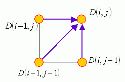
- Local constraint: For any given node $(i, j)$ in the path, the possible fan-in nodes are restricted to $(i-1, j)$, $(i, j-1)$, $(i-1, j-1)$. This local constraint guarantees that the mapping path is monotonically non-decreasing in its first and second arguments. Moreover, for any given element in $\mathbf{t}$, we should be able to find at least one corresponding element in $\mathbf{r}$, and vice versa.
- 局部關係:假設最佳路徑上任一點可以表示成 (i, j),那麼其前一點路徑只有三種可能:(i-1, j), (i, j-1), (i-1, j-1)。此局部關係定義了路徑的連續性,而且也規定了 t 的任一個元素至少對應一個 r 的元素,反之亦然。
How can we find the optimum mapping path in DTW? An obvious choice is forward DP, which can be summarized in the following three steps:
- Optimum-value function: Define $D(i, j)$ as the DTW distance between $t(1:i)$ and $r(1:j)$, with the mapping path starting from $(1, 1)$ to $(i, j)$.
- Recursion: $$ D(i, j)=|t(i) - r(j)| + min \left\{\begin{matrix} D(i-1, j)\\D(i-1, j-1)\\D(i, j-1) \end{matrix}\right\}, $$ with the initial condition $D(1, 1)=|t(1)-r(1)|$.
- Final answer: $D(m, n)$.
但是,我們要如何很快地找到這條最佳路徑呢?我們可以根據 DP 的原理,來將 DTW 描述成下列三個步驟:
- 目標函數之定義:定義 D(i, j) 是 t(1:i) 和 r(1:j) 之間的 DTW 距離,對應的最佳路徑是由 (1, 1) 走到 (i, j)。
- 目標函數之遞迴關係:D(i, j) = ∣t(i) - r(j)∣ + min{D(i-1, j), D(i-1, j-1), D(i, j-1)},其端點條件為 D(1, 1) = ∣t(1) - r(1)∣
- 最後答案:$D(m, n)$.
In practice, we need to construct a matrix D of dimensions m×n first and fill in the value of $D(1, 1)$ by using the initial condition. Then by using the recursive formula, we fill the whole matrix one element at a time, by following a column-by-column or row-by-row order. The final answer will be available as $D(m, n)$, with a computational complexity of $O(mn)$.
在上述的方法描述中,我們是有點濫用數學符號,嚴格地說,D(i, j) 應該表示成為 D(t(1:i), r(1:j)),才能準確地描述 D(•,•) 和 t、r 的關係。另外,D() 具有下列對稱的性質:D(t(1:i), r(1:j)) = D(r(1:j), t(1:i))。
在實際運算時,我們通常事先建立一個矩陣 D,其維度為 m×n,先根據端點條件來填入 D(1, 1),然後再根據遞迴關係,逐行或逐列算出 D(i, j) 的值,最後就可以得到我們所要的答案 D(m, n)。有上述方法可得知,DTW 的計算複雜度大約是 O(mn),比用暴力法是有效率多了。
If we want to know the optimum mapping path in addition to the minimum distance, we may want to keep the optimum fan-in of each node. Then at the end of DP, we can quickly back track to find the optimum mapping path between the two input vectors.
如果我們除了要知道 DTW 距離之外,也希望把相關最佳路徑找出來,此時在計算遞迴關係式時,就要記錄每一個最小點所對應的路徑,直到我們求出 D(m, n),在反覆回推前一個最佳路徑的位置,如此一再反覆,才能算出整個最佳路徑,這個步驟在 DP 裡面稱為 Back Tracking。
We can also have the backward DP for DTW, as follows:
- Optimum-value function: Define $D(i, j)$ as the DTW distance between $t(i:m)$ and $r(j:n)$, with the mapping path from $(i, j)$ to $(m, n)$.
- Recursion: $$ D(i, j) = |t(i) - r(j)| + min\left\{\begin{matrix}D(i+1, j)\\D(i+1, j+1)\\D(i, j+1)\end{matrix}\right\},$$ with the initial condition $D(m, n) =|t(m) - r(n)|$.
- Final answer: $D(1, 1)$.
此外,在上述方法中,我們定義的子路徑是由 (1, 1) 走到 (i, j),我們也可以反向操作,定義子路徑是由 (i, j) 走到 (m, n),此時對應的 DTW 解法可以描述成下列四大步驟:
- 目標函數:定義 D(i, j) 是 t(i:m) 和 r(j:n) 之間的 DTW 距離,對應的最佳路徑是由 (i, j) 走到 (m, n)。
- 遞迴關係:D(i, j) = ∣t(i) - r(j)∣ + min{D(i+1, j), D(i+1, j+1), D(i, j+1)},端點條件為 D(m, n) = ∣t(m) - r(n)∣
- 最後答案:D(1, 1)
Another commonly used local path constraint is to set the fan-in of 27°-45°-63° only, as shown in the following figure:
另一個常用到的 local path constraint,是 27°-45°-63°,如下圖所示:
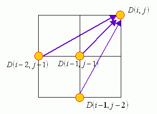
The use of this local path constraint leads to the following potential results:
- Some points in the input vectors could be skipped in the mapping path. This is advantageous if the input vectors contains sporadic outliners.
- Since the optimum-value function is based on the total distance, sometimes the mapping path will take the local paths of 27° or 63° instead of 45° in attempting to minimize the total distance.
此種 local path constraint,會有下列特色:
- 會「跳點」,因此若有一點雜訊,最佳的 DTW 路徑將會跳掉此點。
- 如果最佳路徑是對應於總距離的最小值,那麼最佳路徑會盡量走 27 或 63 度,以使對應到的點數降低。
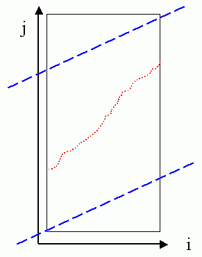
If the required mapping path is "anchored beginning, anchored end", then the local path constraints can induce the global path constraints, as shown next:
如果我們要求是「頭對頭、尾對尾」的比對,那麼由上述的 local path constraint,我們就可以推斷出 global path constraint,如下所示:
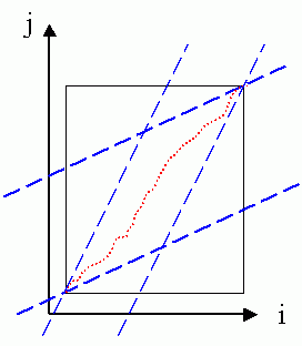
In the above figure, the feasible region for the mapping path is shown as a parallelogram. In filling up the matrix, we can save computation by skipping the elements outside the parallelogram. In addition, a feasible mapping exists only when the ratio of the input vectors' lengths are between 0.5 and 2.
換句話說,若要使 DTW 的比對有意義,那麼兩者長度的比值必須介於 0.5 和 2.0 之間,否則我們就不可能找出一條合法的路徑。如果我們事先能夠定義 global path constraint,那麼在進行 DTW 計算時,就可以省掉很多不需要計算的部分。
If the required mapping path is "anchored beginning and free end" (which is used for query by singing or humming), then the induced global path constraints are shown next:
如果我們要求的是「頭對頭、尾自由」的比對,例如用在「哼唱選歌」的「從頭比對」時,那麼對應的 global path constraint 如下:
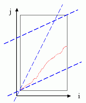
The feasible region for the mapping path is shown as a trapezoid in the above figure. Compared with the case of "anchored beginning and anchored end", we can save less computation by using this set constraints.
這時候可以省略的計算,就會變少。
If the required mapping path is "free beginning and free end" (which is used for speaker-dependent keyword spotting), then the induced global path constraints are shown next:
如果我們要求的是「頭尾都自由」的比對時,對應的 global path constraint 如下:
The feasible region for the mapping path is shown as a parallelogram in the above figure. Compared with the case of "anchored beginning and free end", we can save less computation by using this set constraints.
很明顯的,可以省略的計算,就更少了。
It should be noted that the global path constraints are induced as a result of the local path constraints of 27°-45°-63°. However, when we are using the local path constraints of 0°-45°-90°,sometimes we still apply the global path constraints in order to limit the mapping path to a reasonable shape. In summary, the use of global path constraints serves two purposes:
- Reduce computation load.
- Limit the mapping path to be a reasonable one.
In the following, we shall give some examples of DTW. For simplicity, we shall distinguish two types of DTW:
- Type-1 DTW uses 27°-45°-63° local path constraint.
- Type-2 DTW uses 0°-45°-90° local path constraint.
First, we can use dtw.m (with dtwOpt.type=1) and dtwPathPlot.m to plot the mapping path of type-1 DTW in the following example:
In the above example, we deliberately put an outliner in vec1. Due to the local path constraints of type-1 DTW, this outliner is skipped in the optimum mapping path.
Similarly, we can use dtw.m (with dtwOpt.type=2) and dtwPathPlot.m to plot the mapping path of type-2 DTW:
The outliner cannot be skipped since the local path constraints require each point in a vector has at least one correspondence in the other vector.
By using dtwBridgePlot.m, we can use red lines to connect corresponding points in two vectors, as follows:
It becomes more obvious that type-1 DTW can have empty correspondence while type-2 DTW can have multiple correspondences. Moreover, we can use an extra argument for dtwBridgePlot.m to put the two vectors in 3D space to have a more interesting representation:
Data Clustering and Pattern Recognition (資料分群與樣式辨認)
