Tutorial on leaf recognition
This tutorial covers the basics of leaf recognition based on its shape and color statistics. The dataset is availabe at <http://flavia.sourceforge.net>.
Contents
Preprocessing
Before we start, let's add necessary toolboxes to the search path of MATLAB:
addpath d:/users/jang/matlab/toolbox/utility
addpath d:/users/jang/matlab/toolbox/machineLearning
All the above toolboxes can be downloaded from the author's toolbox page. Make sure you are using the latest toolboxes to work with this script.
For compatibility, here we list the platform and MATLAB version that we used to run this script:
fprintf('Platform: %s\n', computer);
fprintf('MATLAB version: %s\n', version);
fprintf('Date & time: %s\n', char(datetime));
scriptStartTime=tic;
Platform: PCWIN64
MATLAB version: 9.3.0.651671 (R2017b) Prerelease
Date & time: 18-Jan-2018 07:39:39
Dataset construction
First of all, we shall collect all the image data from the image directory. Note that
- The images have been reorganized for easy parsing (with a subfolder for each class), which can be downloaded from here.
- For simplicity, we shall only use 5 classes instead of the original 32 classes.
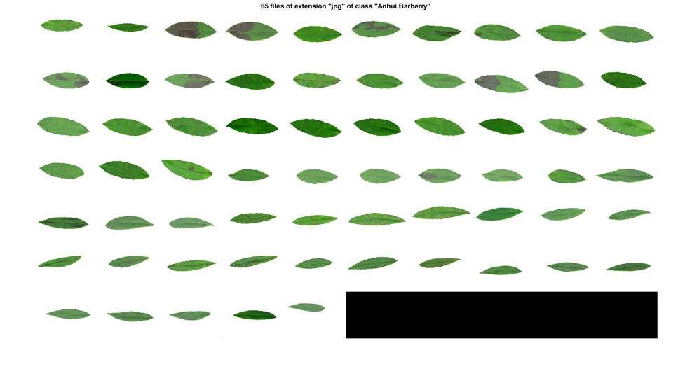
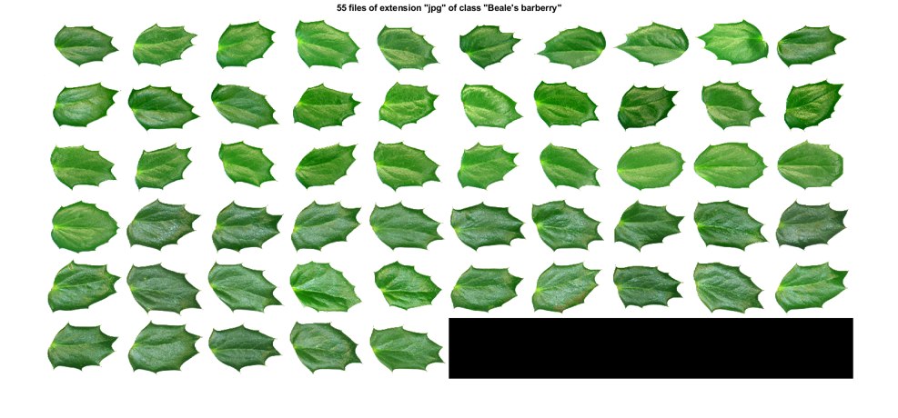
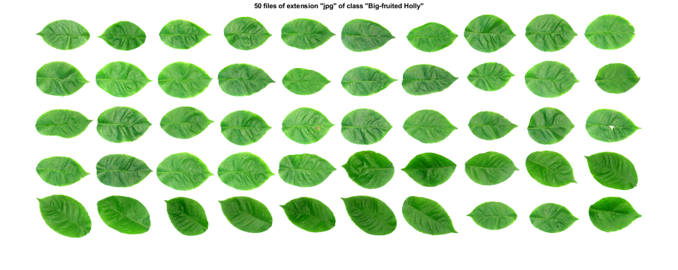
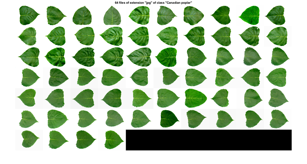
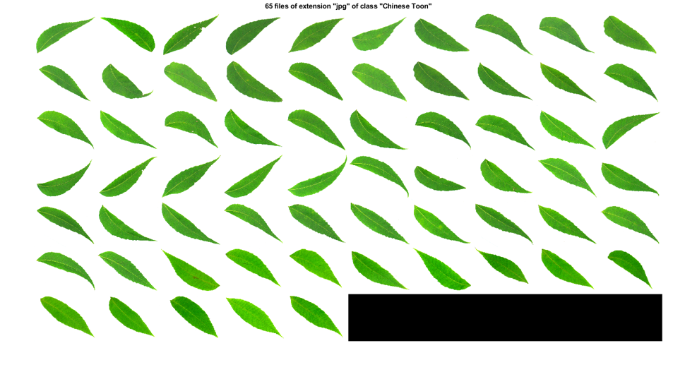
- During the data collection, we shall also plot the leaves for each class.
imDir='D:\users\jang\books\dcpr\appNote\leafId\leafSorted';
opt=mmDataCollect('defaultOpt');
opt.extName='jpg';
opt.maxClassNum=5;
imageData=mmDataCollect(imDir, opt, 1);
Collecting 299 files with extension "jpg" from "D:\users\jang\books\dcpr\appNote\leafId\leafSorted"...
Warning: Image is too big to fit on screen; displaying at 13%
Warning: Image is too big to fit on screen; displaying at 13%
Warning: Image is too big to fit on screen; displaying at 13%
Warning: Image is too big to fit on screen; displaying at 13%
Warning: Image is too big to fit on screen; displaying at 13%
Feature extraction
For each image, we need to extract the corresponding features for classification. We shall use the function "leafFeaExtract" for feature extraction. We also need to put all the dataset into a format that is easier for further processing, including classifier construction and evaluation.
opt=dsCreateFromMm('defaultOpt');
if exist('ds.mat', 'file')
	fprintf('Loading ds.mat...\n');
	load ds.mat
else
	myTic=tic;
	opt=dsCreateFromMm('defaultOpt');
	opt.imFeaFcn=@leafFeaExtract;	% Function for feature extraction
	opt.imFeaOpt=feval(opt.imFeaFcn, 'defaultOpt');	% Feature options
	ds=dsCreateFromMm(imageData, opt);
	fprintf('Time for feature extraction over %d images = %g sec\n', length(imageData), toc(myTic));
	fprintf('Saving ds.mat...\n');
	save ds ds
end
Loading ds.mat...
Note that since feature extraction is a lengthy process, we have save the resulting variable "ds" into "ds.mat". If needed, you can simply load the file to restore the dataset variable "ds" and play around with it. But if you have changed the feature extraction function, be sure to delete ds.mat first to enforce the feature extraction.
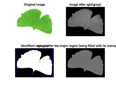
Basically the extracted features are based on the regions separated by Otsu's method. We only consider the region with the maximum area, and compute its region properties and color statistics as features. You can type "leafFeaExtract" to have a self-demo of the function:
figure; leafFeaExtract;
Dataset visualization
Once we have all the necessary information stored in "ds", we can invoke many different functions in Machine Learning Toolbox for data visualization and classification.
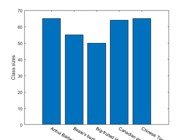
For instance, we can display the size of each class:
figure;
[classSize, classLabel]=dsClassSize(ds, 1);
6 features
299 instances
5 classes
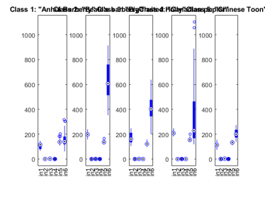
We can plot the distribution of each features within each class:
figure; dsBoxPlot(ds);
The box plots indicate the ranges of the features vary a lot. To verify this, we can simply plot the range of features of the dataset:
figure; dsRangePlot(ds);
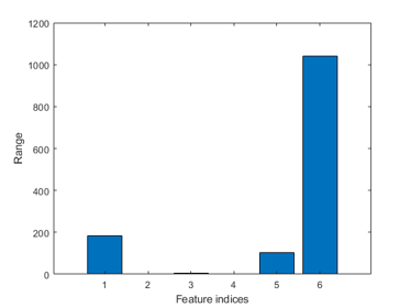
Big range difference cause problems in distance-based classification. To avoid this, we can simply apply z-normalization to each feature:
ds2=ds;
ds2.input=inputNormalize(ds2.input);
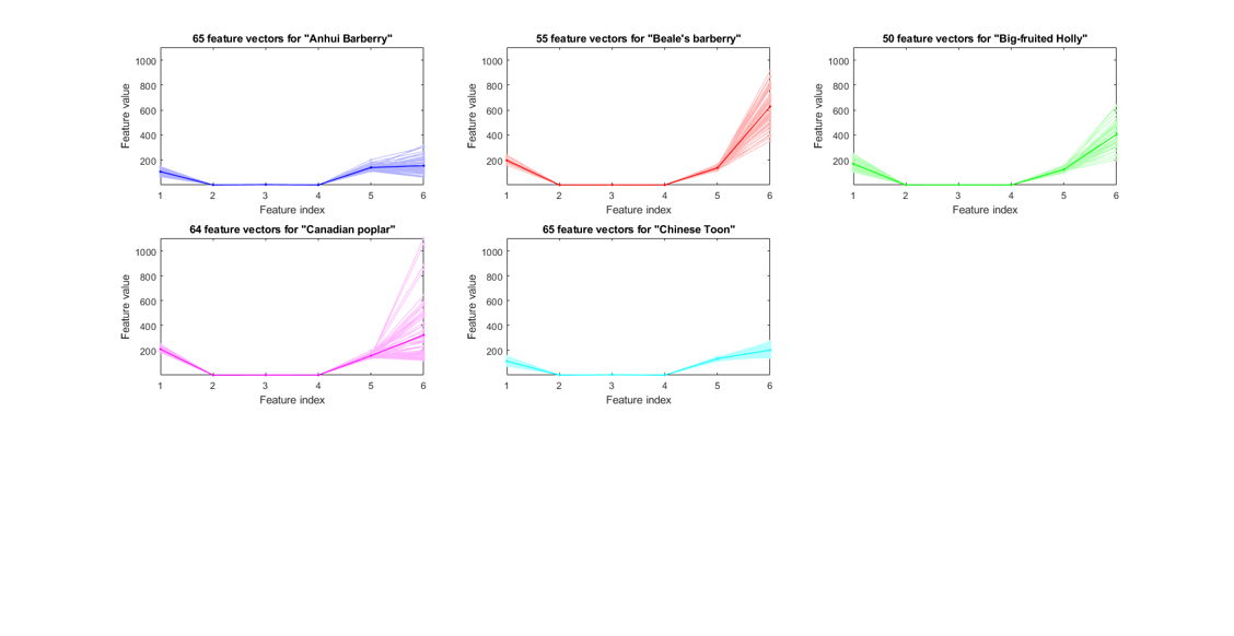
We can now plot the feature vectors within each class:
figure; dsFeaVecPlot(ds); figEnlarge;
We can also do scatter plots on each pair of the original features:
figure; dsProjPlot2(ds); figEnlarge;
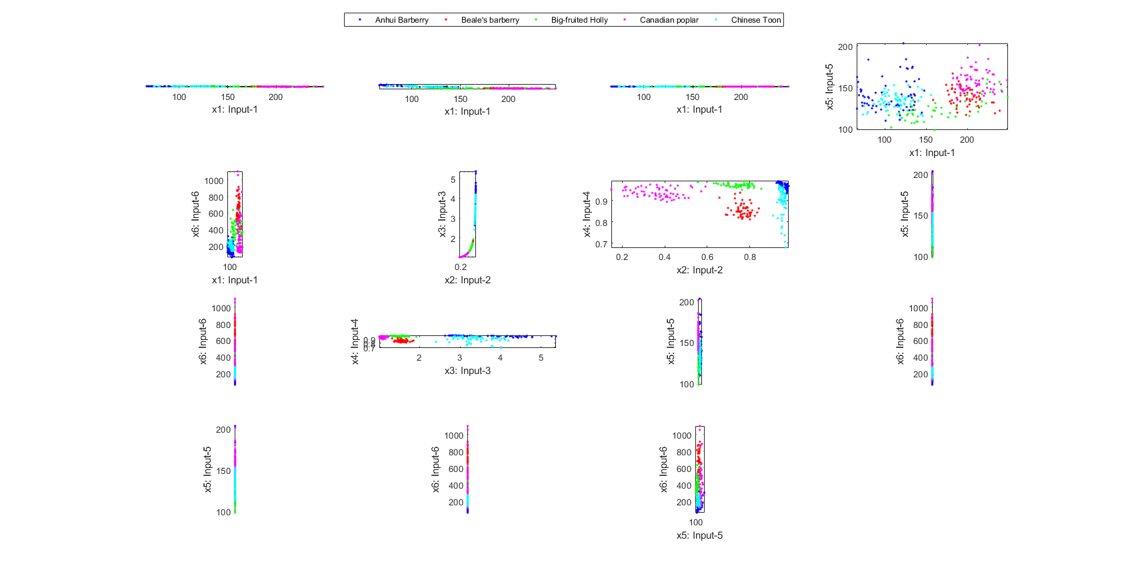
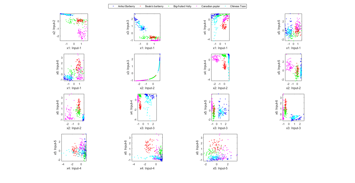
It is hard to see the above plots due to a large difference in the range of each features. We can try the same plot with normalized inputs:
figure; dsProjPlot2(ds2); figEnlarge;
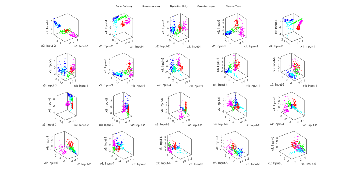
We can also do the scatter plots in the 3D space:
figure; dsProjPlot3(ds2); figEnlarge;
In order to visualize the distribution of the dataset, we can project the original dataset into 2-D space. This can be achieved by LDA (linear discriminant analysis):
ds2d=lda(ds);
ds2d.input=ds2d.input(1:2, :);
figure; dsScatterPlot(ds2d); xlabel('Input 1'); ylabel('Input 2');
title('Features projected on the first 2 lda vectors');

Classification
We can try the most straightforward KNNC (k-nearest neighbor classifier):
rr=knncLoo(ds);
fprintf('rr=%g%% for ds\n', rr*100);
rr=77.2575% for ds
For normalized dataset, usually we can obtain a better accuracy:
[rr, computed]=knncLoo(ds2);
fprintf('rr=%g%% for ds2 of normalized inputs\n', rr*100);
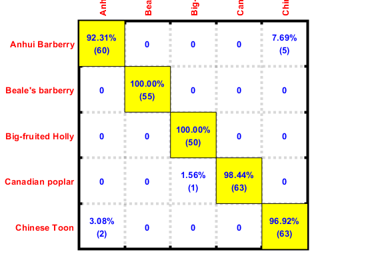
rr=97.3244% for ds2 of normalized inputs
We can plot the confusion matrix:
confMat=confMatGet(ds2.output, computed);
opt=confMatPlot('defaultOpt');
opt.className=ds.outputName;
opt.mode='both';
figure; confMatPlot(confMat, opt);
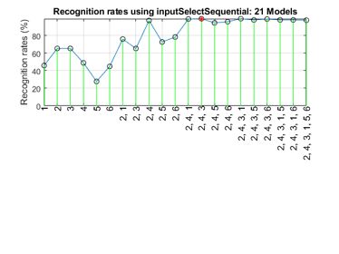
We can perform sequential input selection to find the best features:
figure; tic; inputSelectSequential(ds2, inf, 'knnc'); toc
Construct 21 knnc models, each with up to 6 inputs selected from 6 candidates...

Selecting input 1:
Model 1/21: selected={1} => Recog. rate = 45.8%
Model 2/21: selected={2} => Recog. rate = 65.2%
Model 3/21: selected={3} => Recog. rate = 65.2%
Model 4/21: selected={4} => Recog. rate = 48.8%
Model 5/21: selected={5} => Recog. rate = 27.8%
Model 6/21: selected={6} => Recog. rate = 44.8%
Currently selected inputs: 2

Selecting input 2:
Model 7/21: selected={2, 1} => Recog. rate = 75.9%
Model 8/21: selected={2, 3} => Recog. rate = 65.2%
Model 9/21: selected={2, 4} => Recog. rate = 97.0%
Model 10/21: selected={2, 5} => Recog. rate = 72.6%
Model 11/21: selected={2, 6} => Recog. rate = 78.3%
Currently selected inputs: 2, 4

Selecting input 3:
Model 12/21: selected={2, 4, 1} => Recog. rate = 98.7%
Model 13/21: selected={2, 4, 3} => Recog. rate = 99.0%
Model 14/21: selected={2, 4, 5} => Recog. rate = 94.3%
Model 15/21: selected={2, 4, 6} => Recog. rate = 95.7%
Currently selected inputs: 2, 4, 3

Selecting input 4:
Model 16/21: selected={2, 4, 3, 1} => Recog. rate = 99.0%
Model 17/21: selected={2, 4, 3, 5} => Recog. rate = 97.7%
Model 18/21: selected={2, 4, 3, 6} => Recog. rate = 98.7%
Currently selected inputs: 2, 4, 3, 1

Selecting input 5:
Model 19/21: selected={2, 4, 3, 1, 5} => Recog. rate = 97.7%
Model 20/21: selected={2, 4, 3, 1, 6} => Recog. rate = 97.7%
Currently selected inputs: 2, 4, 3, 1, 5

Selecting input 6:
Model 21/21: selected={2, 4, 3, 1, 5, 6} => Recog. rate = 97.3%
Currently selected inputs: 2, 4, 3, 1, 5, 6

Overall maximal recognition rate = 99.0%.
Selected 3 inputs (out of 6): 2, 4, 3
Elapsed time is 0.316317 seconds.
Since the number of features is not too big, we can also exhaustive search to find the best features:
figure; tic; inputSelectExhaustive(ds2, inf, 'knnc'); toc
Construct 63 knnc models, each with up to 6 inputs selected from 6 candidates...
modelIndex 1/63: selected={1} => Recog. rate = 45.819398%
modelIndex 2/63: selected={2} => Recog. rate = 65.217391%
modelIndex 3/63: selected={3} => Recog. rate = 65.217391%
modelIndex 4/63: selected={4} => Recog. rate = 48.829431%
modelIndex 5/63: selected={5} => Recog. rate = 27.759197%
modelIndex 6/63: selected={6} => Recog. rate = 44.816054%
modelIndex 7/63: selected={1, 2} => Recog. rate = 75.919732%
modelIndex 8/63: selected={1, 3} => Recog. rate = 77.257525%
modelIndex 9/63: selected={1, 4} => Recog. rate = 88.628763%
modelIndex 10/63: selected={1, 5} => Recog. rate = 59.531773%
modelIndex 11/63: selected={1, 6} => Recog. rate = 73.913043%
modelIndex 12/63: selected={2, 3} => Recog. rate = 65.217391%
modelIndex 13/63: selected={2, 4} => Recog. rate = 96.989967%
modelIndex 14/63: selected={2, 5} => Recog. rate = 72.575251%
modelIndex 15/63: selected={2, 6} => Recog. rate = 78.260870%
modelIndex 16/63: selected={3, 4} => Recog. rate = 99.331104%
modelIndex 17/63: selected={3, 5} => Recog. rate = 72.240803%
modelIndex 18/63: selected={3, 6} => Recog. rate = 79.933110%
modelIndex 19/63: selected={4, 5} => Recog. rate = 63.210702%
modelIndex 20/63: selected={4, 6} => Recog. rate = 74.247492%
modelIndex 21/63: selected={5, 6} => Recog. rate = 59.531773%
modelIndex 22/63: selected={1, 2, 3} => Recog. rate = 77.591973%
modelIndex 23/63: selected={1, 2, 4} => Recog. rate = 98.662207%
modelIndex 24/63: selected={1, 2, 5} => Recog. rate = 80.267559%
modelIndex 25/63: selected={1, 2, 6} => Recog. rate = 85.284281%
modelIndex 26/63: selected={1, 3, 4} => Recog. rate = 98.662207%
modelIndex 27/63: selected={1, 3, 5} => Recog. rate = 78.595318%
modelIndex 28/63: selected={1, 3, 6} => Recog. rate = 85.953177%
modelIndex 29/63: selected={1, 4, 5} => Recog. rate = 88.963211%
modelIndex 30/63: selected={1, 4, 6} => Recog. rate = 93.645485%
modelIndex 31/63: selected={1, 5, 6} => Recog. rate = 79.598662%
modelIndex 32/63: selected={2, 3, 4} => Recog. rate = 98.996656%
modelIndex 33/63: selected={2, 3, 5} => Recog. rate = 72.575251%
modelIndex 34/63: selected={2, 3, 6} => Recog. rate = 79.264214%
modelIndex 35/63: selected={2, 4, 5} => Recog. rate = 94.314381%
modelIndex 36/63: selected={2, 4, 6} => Recog. rate = 95.652174%
modelIndex 37/63: selected={2, 5, 6} => Recog. rate = 80.602007%
modelIndex 38/63: selected={3, 4, 5} => Recog. rate = 97.658863%
modelIndex 39/63: selected={3, 4, 6} => Recog. rate = 98.996656%
modelIndex 40/63: selected={3, 5, 6} => Recog. rate = 81.270903%
modelIndex 41/63: selected={4, 5, 6} => Recog. rate = 79.598662%
modelIndex 42/63: selected={1, 2, 3, 4} => Recog. rate = 98.996656%
modelIndex 43/63: selected={1, 2, 3, 5} => Recog. rate = 80.602007%
modelIndex 44/63: selected={1, 2, 3, 6} => Recog. rate = 87.959866%
modelIndex 45/63: selected={1, 2, 4, 5} => Recog. rate = 97.658863%
modelIndex 46/63: selected={1, 2, 4, 6} => Recog. rate = 98.327759%
modelIndex 47/63: selected={1, 2, 5, 6} => Recog. rate = 85.618729%
modelIndex 48/63: selected={1, 3, 4, 5} => Recog. rate = 96.989967%
modelIndex 49/63: selected={1, 3, 4, 6} => Recog. rate = 96.989967%
modelIndex 50/63: selected={1, 3, 5, 6} => Recog. rate = 85.953177%
modelIndex 51/63: selected={1, 4, 5, 6} => Recog. rate = 95.652174%
modelIndex 52/63: selected={2, 3, 4, 5} => Recog. rate = 97.658863%
modelIndex 53/63: selected={2, 3, 4, 6} => Recog. rate = 98.662207%
modelIndex 54/63: selected={2, 3, 5, 6} => Recog. rate = 83.612040%
modelIndex 55/63: selected={2, 4, 5, 6} => Recog. rate = 93.645485%
modelIndex 56/63: selected={3, 4, 5, 6} => Recog. rate = 96.655518%
modelIndex 57/63: selected={1, 2, 3, 4, 5} => Recog. rate = 97.658863%
modelIndex 58/63: selected={1, 2, 3, 4, 6} => Recog. rate = 97.658863%
modelIndex 59/63: selected={1, 2, 3, 5, 6} => Recog. rate = 89.297659%
modelIndex 60/63: selected={1, 2, 4, 5, 6} => Recog. rate = 97.993311%
modelIndex 61/63: selected={1, 3, 4, 5, 6} => Recog. rate = 95.986622%
modelIndex 62/63: selected={2, 3, 4, 5, 6} => Recog. rate = 98.327759%
modelIndex 63/63: selected={1, 2, 3, 4, 5, 6} => Recog. rate = 97.324415%

Overall max recognition rate = 99.3%.
Selected 2 inputs (out of 6): 3, 4
Elapsed time is 0.554176 seconds.
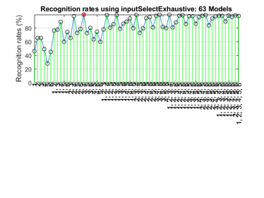
It is obvious that the exhaustive search can find the best features, but at the cost of more computation.
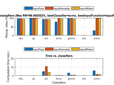
We can even perform an exhaustive search on the classifiers and the way of input normalization:
opt=perfCv4classifier('defaultOpt');
opt.foldNum=10;
tic; [perfData, bestId]=perfCv4classifier(ds, opt, 1); toc
structDispInHtml(perfData, 'Performance of various classifiers via cross validation');
Warning in gmmTrain: max(range)/min(range)=10881.1>10000 ===> Perhaps you should normalize the data first.
Warning in gmmTrain: max(range)/min(range)=13356.6>10000 ===> Perhaps you should normalize the data first.
Warning in gmmTrain: max(range)/min(range)=12241.4>10000 ===> Perhaps you should normalize the data first.
Warning in gmmTrain: max(range)/min(range)=12103.1>10000 ===> Perhaps you should normalize the data first.
Warning in gmmTrain: max(range)/min(range)=10881.1>10000 ===> Perhaps you should normalize the data first.
Warning in gmmTrain: max(range)/min(range)=12103.1>10000 ===> Perhaps you should normalize the data first.
Warning in gmmTrain: max(range)/min(range)=10881.1>10000 ===> Perhaps you should normalize the data first.
Warning in gmmTrain: max(range)/min(range)=11780.9>10000 ===> Perhaps you should normalize the data first.
Warning in gmmTrain: max(range)/min(range)=10289.8>10000 ===> Perhaps you should normalize the data first.
Warning in gmmTrain: max(range)/min(range)=12103.1>10000 ===> Perhaps you should normalize the data first.
Warning in gmmTrain: max(range)/min(range)=10881.1>10000 ===> Perhaps you should normalize the data first.
Warning in gmmTrain: max(range)/min(range)=12103.1>10000 ===> Perhaps you should normalize the data first.
Warning in gmmTrain: max(range)/min(range)=10775.2>10000 ===> Perhaps you should normalize the data first.
Warning in gmmTrain: max(range)/min(range)=12103.1>10000 ===> Perhaps you should normalize the data first.
Warning in gmmTrain: max(range)/min(range)=10881.1>10000 ===> Perhaps you should normalize the data first.
Warning in gmmTrain: max(range)/min(range)=12103.1>10000 ===> Perhaps you should normalize the data first.
Warning in gmmTrain: max(range)/min(range)=10881.1>10000 ===> Perhaps you should normalize the data first.
Warning in gmmTrain: max(range)/min(range)=12103.1>10000 ===> Perhaps you should normalize the data first.
Warning in gmmTrain: max(range)/min(range)=12279.3>10000 ===> Perhaps you should normalize the data first.
Warning in gmmTrain: max(range)/min(range)=12084.8>10000 ===> Perhaps you should normalize the data first.
Elapsed time is 34.157843 seconds.
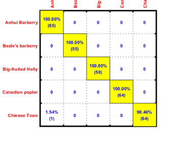
We can then display the confusion matrix of the best classifier:
confMat=confMatGet(ds.output, perfData(bestId).bestComputedClass);
opt=confMatPlot('defaultOpt');
opt.className=ds.outputName;
figure; confMatPlot(confMat, opt);
We can also list all the misclassified images in a table:
for i=1:length(imageData)
	imageData(i).classIdPredicted=perfData(bestId).bestComputedClass(i);
	imageData(i).classPredicted=ds.outputName{imageData(i).classIdPredicted};
end
listOpt=mmDataList('defaultOpt');
mmDataList(imageData, listOpt);
| Index\Field | File | GT ==> Predicted | Hit | url |
|---|---|---|---|---|
| 1 | 3173.jpg | Chinese Toon ==> Anhui Barberry | false | 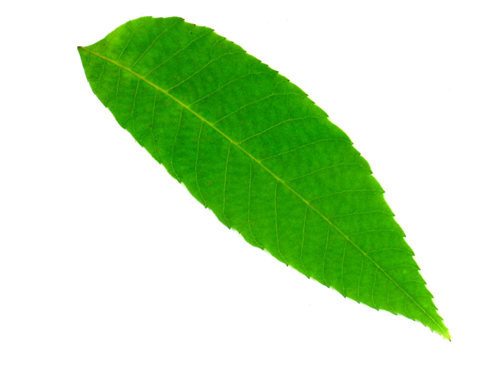 |
Summary
This is a brief tutorial on leaf recognition based on its shape and color statistics. There are several directions for further improvement:
- Explore other features, such as vein distribution
- Try the classification problem using the whole dataset
- Use template matching as an alternative to improve the performance
Appendix
List of functions, scripts, and datasets used in this script:
- Dataset used in this script.
- List of files in this folder
Overall elapsed time:
toc(scriptStartTime)
Elapsed time is 79.447077 seconds.
Jyh-Shing Roger Jang, created on
datetime
ans =

  datetime

   18-Jan-2018 07:40:58
If you are interested in the original MATLAB code for this page, you can type "grabcode(URL)" under MATLAB, where URL is the web address of this page.