Tutorial on human recognition

In this tutorial, we shall explain the basics of human recognition based on its shape. The dataset is availabe at <http://mirlab.org/jang/books/dcpr/appNote/humanId/humanDataset.rar>.

Preprocessing
Dataset construction
Feature extraction
Dataset visualization
Classification
Summary

Preprocessing

Before we start, let's add necessary toolboxes to the search path of MATLAB:

addpath d:/users/jang/matlab/toolbox/utility
addpath d:/users/jang/matlab/toolbox/machineLearning

For compatibility, here we list the platform and MATLAB version that we used to run this script:

fprintf('Platform: %s\n', computer);
fprintf('MATLAB version: %s\n', version);
scriptStartTime=tic;

Platform: PCWIN64
MATLAB version: 8.3.0.532 (R2014a)

Dataset construction

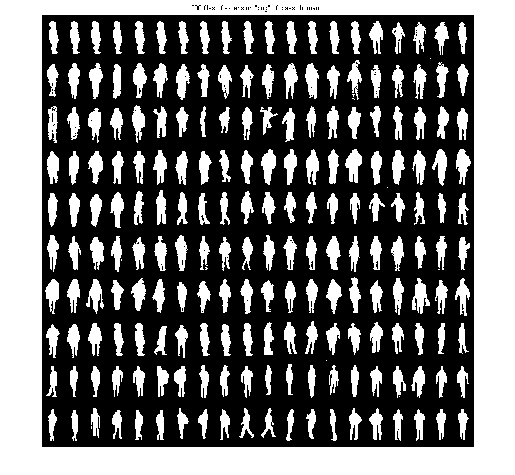
First of all, we shall collect all the image data from the image directory. Note that

The images have been reorganized for easy parsing, with a subfolder for each class.
During the data collection, we shall also plot the images for each class.

imDir='D:\users\jang\books\dcpr\appNote\humanId\humanDataset';
opt=mmDataCollect('defaultOpt');
opt.extName='png';
opt.montageSize=[nan, 20];
imageData=mmDataCollect(imDir, opt, 1);

Collecting 400 files with extension "png" from "D:\users\jang\books\dcpr\appNote\humanId\humanDataset"...
Warning: Image is too big to fit on screen; displaying at 67% 
Warning: Image is too big to fit on screen; displaying at 67%

Feature extraction

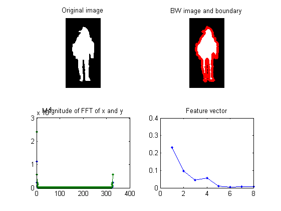
For each image, we need to extract the corresponding feature vector for classification. We shall use the function humanFeaExtract.m (which computes the Fourier descriptors of the object's boundary) for feature extraction. We also need to put all the dataset into a format that is easier for further processing, including classifier construction and evaluation.

myTic=tic;
opt=dsCreateFromMm('defaultOpt');
opt.imFeaFcn=@humanFeaExtract;	% Function for feature extraction
opt.imFeaOpt=feval(opt.imFeaFcn, 'defaultOpt');	% Feature options
ds=dsCreateFromMm(imageData, opt);
fprintf('Time for feature extraction over %d images = %g sec\n', length(imageData), toc(myTic));
fprintf('Saving ds.mat...\n');

Extracting features from each multimedia object...
100/400: file=D:\users\jang\books\dcpr\appNote\humanId\humanDataset/human/TrainingDatas300.png, time=0.00165416 sec
200/400: file=D:\users\jang\books\dcpr\appNote\humanId\humanDataset/human/TrainingDatas400.png, time=0.00134539 sec
300/400: file=D:\users\jang\books\dcpr\appNote\humanId\humanDataset/nonHuman/TrainingDatas189.png, time=0.00164133 sec
400/400: file=D:\users\jang\books\dcpr\appNote\humanId\humanDataset/nonHuman/TrainingDatas99.png, time=0.00137533 sec
Time for feature extraction over 400 images = 0.631754 sec
Saving ds.mat...

Note that if feature extraction is lengthy, we can simply load ds.mat which has been save in the above code snippet.

Basically the extracted features are based on the shape of the object. You can type "humanFeaExtract" to have a self-demo of the function:

figure; humanFeaExtract;

Dataset visualization

Once we have every piece of necessary information stored in "ds", we can invoke many different functions in Machine Learning Toolbox for data visualization and classification.

For instance, we can display the size of each class:

figure;
[classSize, classLabel]=dsClassSize(ds, 1);

8 features
400 instances
2 classes

We can plot the distribution of each features within each class:

figure; dsBoxPlot(ds);

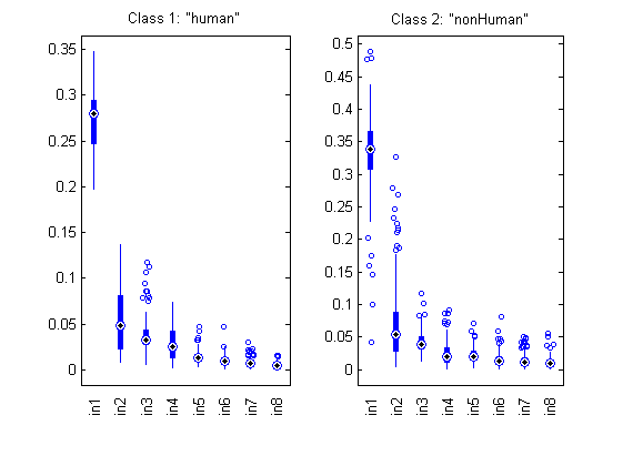
The box plots indicate the ranges of the features vary a lot. To verify, we can simply plot the range of features of the dataset:

figure; dsRangePlot(ds);

Big range difference cause problems in distance-based classification. To avoid this, we can simply normalize the features:

ds2=ds;
ds2.input=inputNormalize(ds2.input);

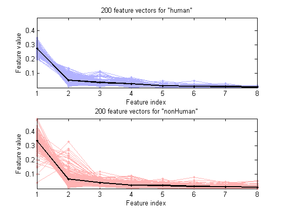
We can plot the feature vectors within each class:

figure; dsFeaVecPlot(ds);

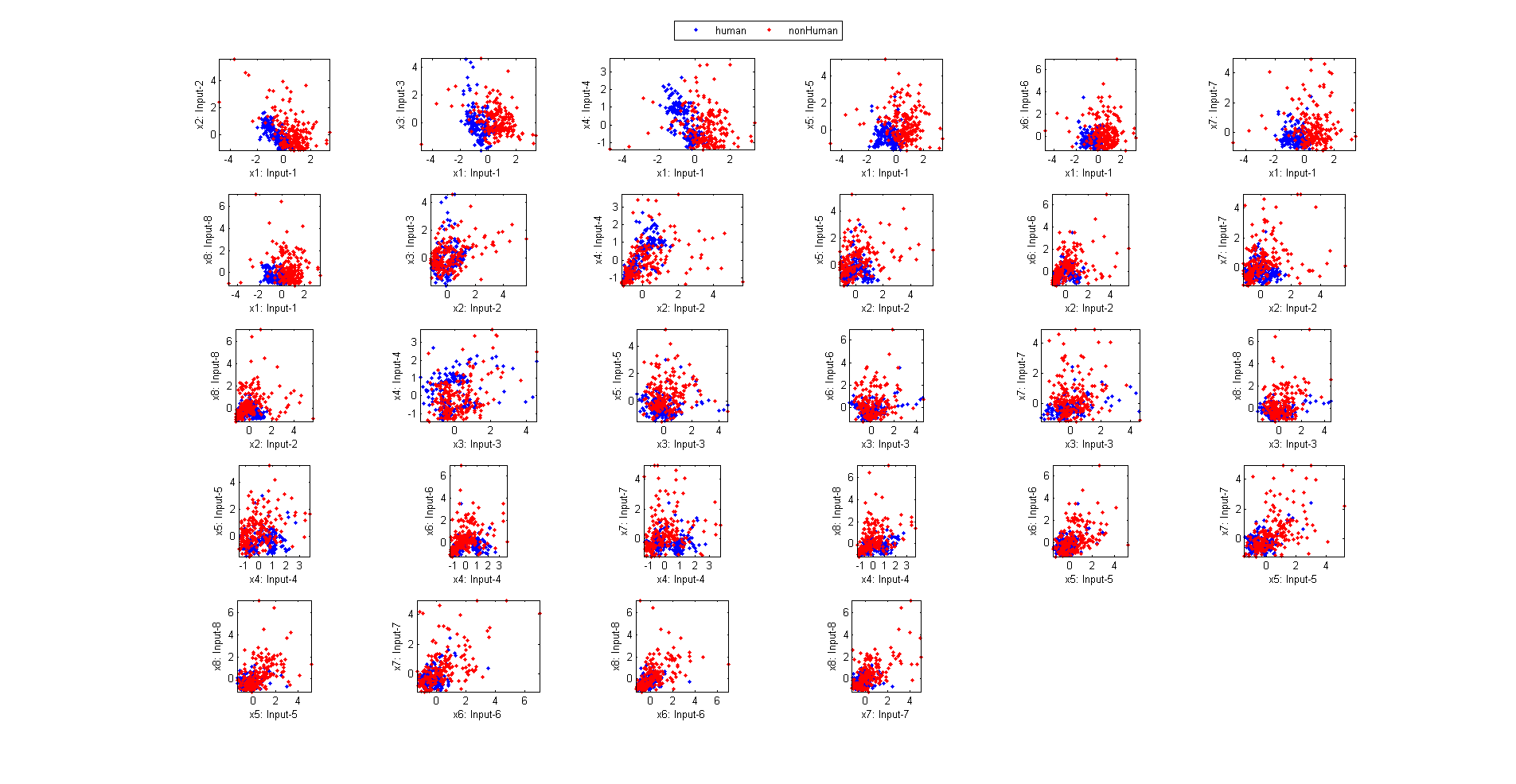
We can do the scatter plots on every 2 features:

figure; dsProjPlot2(ds); figEnlarge;

If the ranges of features vary a lot, we can try the same plot with z-normalized inputs:

figure; dsProjPlot2(ds2); figEnlarge;

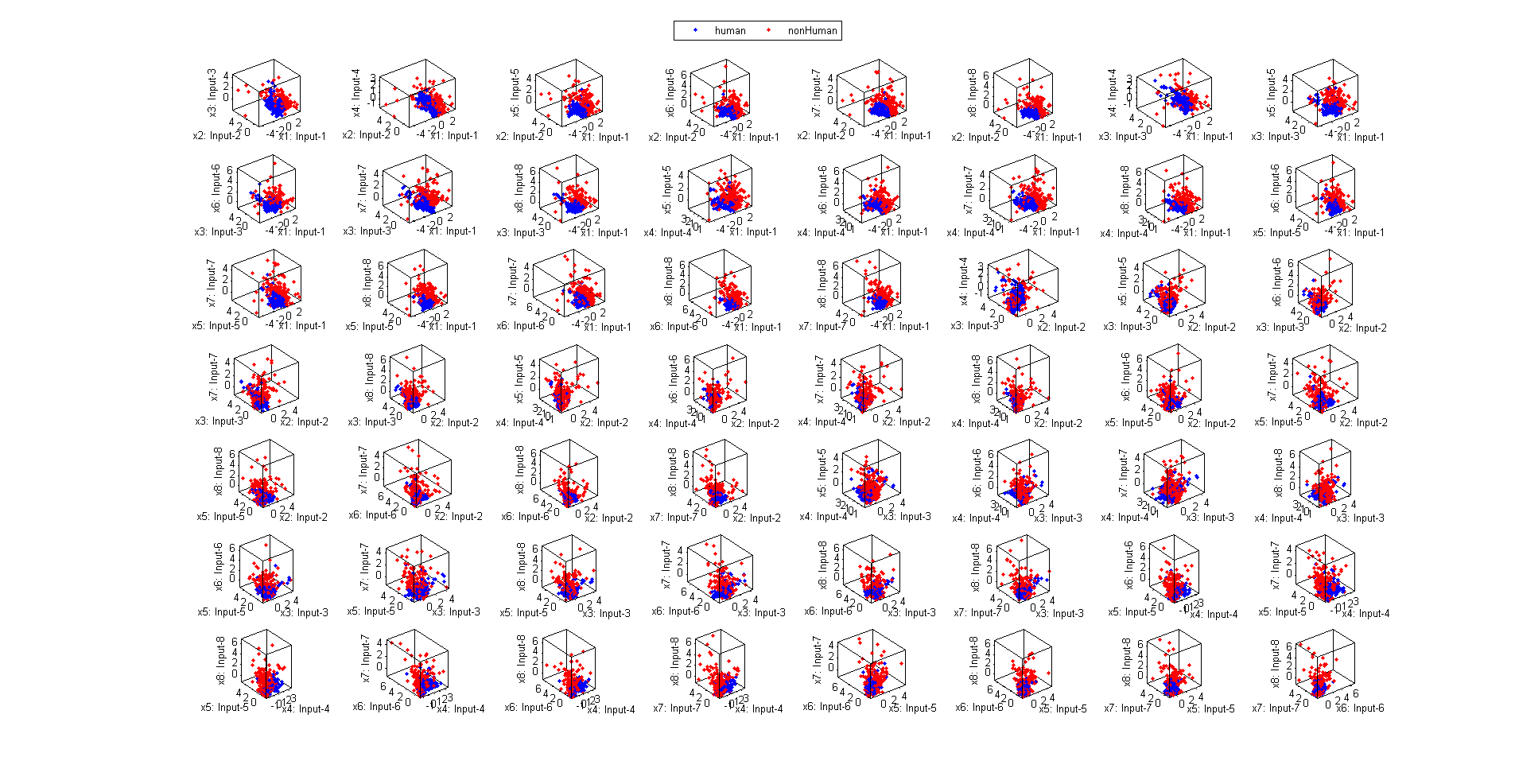
We can also do the scatter plots in the 3D space:

figure; dsProjPlot3(ds2); figEnlarge;

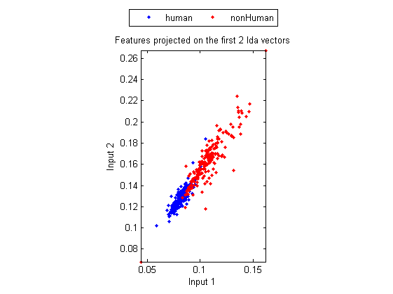
In order to visualize the distribution of the dataset, we can project the original dataset into 2-D space. This can be achieved by LDA (linear discriminant analysis):

ds2d=lda(ds);
ds2d.input=ds2d.input(1:2, :);
figure; dsScatterPlot(ds2d); xlabel('Input 1'); ylabel('Input 2');
title('Features projected on the first 2 lda vectors');

Classification

We can try the most straightforward KNNC (k-nearest neighbor classifier):

rr=knncLoo(ds);
fprintf('rr=%g%% for ds\n', rr*100);

rr=88.5% for ds

For normalized dataset, usually we can obtain a better accuracy:

[rr, computed]=knncLoo(ds2);
fprintf('rr=%g%% for ds2 of normalized inputs\n', rr*100);

rr=91% for ds2 of normalized inputs

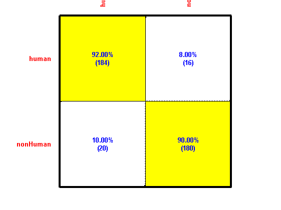
We can plot the confusion matrix:

confMat=confMatGet(ds2.output, computed);
opt=confMatPlot('defaultOpt');
opt.className=ds.outputName;
opt.mode='both';
figure; confMatPlot(confMat, opt);

We can perform input selection to find the best features:

figure; tic; inputSelectSequential(ds2, inf, 'knnc', 1); toc

Construct 36 KNN models, each with up to 8 inputs selected from 8 candidates...

Selecting input 1:
Model 1/36: selected={1} => Recog. rate = 75.5%
Model 2/36: selected={2} => Recog. rate = 54.8%
Model 3/36: selected={3} => Recog. rate = 55.0%
Model 4/36: selected={4} => Recog. rate = 58.5%
Model 5/36: selected={5} => Recog. rate = 58.3%
Model 6/36: selected={6} => Recog. rate = 61.0%
Model 7/36: selected={7} => Recog. rate = 60.8%
Model 8/36: selected={8} => Recog. rate = 61.5%
Currently selected inputs: 1

Selecting input 2:
Model 9/36: selected={1, 2} => Recog. rate = 82.8%
Model 10/36: selected={1, 3} => Recog. rate = 78.8%
Model 11/36: selected={1, 4} => Recog. rate = 80.5%
Model 12/36: selected={1, 5} => Recog. rate = 82.3%
Model 13/36: selected={1, 6} => Recog. rate = 82.0%
Model 14/36: selected={1, 7} => Recog. rate = 80.3%
Model 15/36: selected={1, 8} => Recog. rate = 85.0%
Currently selected inputs: 1, 8

Selecting input 3:
Model 16/36: selected={1, 8, 2} => Recog. rate = 86.0%
Model 17/36: selected={1, 8, 3} => Recog. rate = 86.0%
Model 18/36: selected={1, 8, 4} => Recog. rate = 84.8%
Model 19/36: selected={1, 8, 5} => Recog. rate = 83.5%
Model 20/36: selected={1, 8, 6} => Recog. rate = 85.0%
Model 21/36: selected={1, 8, 7} => Recog. rate = 86.8%
Currently selected inputs: 1, 8, 7

Selecting input 4:
Model 22/36: selected={1, 8, 7, 2} => Recog. rate = 87.5%
Model 23/36: selected={1, 8, 7, 3} => Recog. rate = 87.5%
Model 24/36: selected={1, 8, 7, 4} => Recog. rate = 87.5%
Model 25/36: selected={1, 8, 7, 5} => Recog. rate = 87.3%
Model 26/36: selected={1, 8, 7, 6} => Recog. rate = 86.5%
Currently selected inputs: 1, 8, 7, 2

Selecting input 5:
Model 27/36: selected={1, 8, 7, 2, 3} => Recog. rate = 88.5%
Model 28/36: selected={1, 8, 7, 2, 4} => Recog. rate = 89.5%
Model 29/36: selected={1, 8, 7, 2, 5} => Recog. rate = 89.5%
Model 30/36: selected={1, 8, 7, 2, 6} => Recog. rate = 89.8%
Currently selected inputs: 1, 8, 7, 2, 6

Selecting input 6:
Model 31/36: selected={1, 8, 7, 2, 6, 3} => Recog. rate = 89.3%
Model 32/36: selected={1, 8, 7, 2, 6, 4} => Recog. rate = 90.0%
Model 33/36: selected={1, 8, 7, 2, 6, 5} => Recog. rate = 89.5%
Currently selected inputs: 1, 8, 7, 2, 6, 4

Selecting input 7:
Model 34/36: selected={1, 8, 7, 2, 6, 4, 3} => Recog. rate = 90.0%
Model 35/36: selected={1, 8, 7, 2, 6, 4, 5} => Recog. rate = 91.3%
Currently selected inputs: 1, 8, 7, 2, 6, 4, 5

Selecting input 8:
Model 36/36: selected={1, 8, 7, 2, 6, 4, 5, 3} => Recog. rate = 91.0%
Currently selected inputs: 1, 8, 7, 2, 6, 4, 5, 3

Overall maximal recognition rate = 91.3%.
Selected 7 inputs (out of 8): 1, 8, 7, 2, 6, 4, 5
Elapsed time is 102.044293 seconds.

We can even perform an exhaustive search on the classifiers and input normalization methods:

opt=perfCv4classifier('defaultOpt');
opt.foldNum=10;
tic; [perfData, bestId]=perfCv4classifier(ds, opt, 1); toc
structDispInHtml(perfData, 'Performance of various classifiers via cross validation');

Iteration=200/1000, recog. rate=50%
Iteration=400/1000, recog. rate=69.4444%
Iteration=600/1000, recog. rate=70.5556%
Iteration=800/1000, recog. rate=70.8333%
Iteration=1000/1000, recog. rate=72.2222%
Iteration=200/1000, recog. rate=82.2222%
Iteration=400/1000, recog. rate=89.4444%
Iteration=600/1000, recog. rate=89.1667%
Iteration=800/1000, recog. rate=89.1667%
Iteration=1000/1000, recog. rate=89.1667%
Iteration=200/1000, recog. rate=68.8889%
Iteration=400/1000, recog. rate=90.2778%
Iteration=600/1000, recog. rate=90%
Iteration=800/1000, recog. rate=90%
Iteration=1000/1000, recog. rate=90%
Elapsed time is 25.939329 seconds.

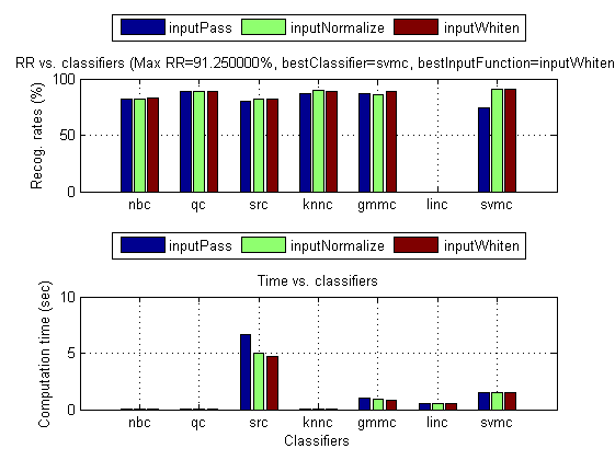
We can then display the confusion matrix of the best classifier:

confMat=confMatGet(ds.output, perfData(bestId).bestComputedClass);
opt=confMatPlot('defaultOpt');
opt.className=ds.outputName;
figure; confMatPlot(confMat, opt);

We can also list all the misclassified images in a table for easy error analysis:

for i=1:length(imageData)
	imageData(i).classIdPredicted=perfData(bestId).bestComputedClass(i);
	imageData(i).classPredicted=ds.outputName{imageData(i).classIdPredicted};
end
listOpt=mmDataList('defaultOpt');
mmDataList(imageData, listOpt);

List of 35 misclassified cases
Index\Field	File	GT ==> Predicted	Hit
1	TrainingDatas239.png	human ==> nonHuman	false
2	TrainingDatas245.png	human ==> nonHuman	false
3	TrainingDatas246.png	human ==> nonHuman	false
4	TrainingDatas251.png	human ==> nonHuman	false
5	TrainingDatas271.png	human ==> nonHuman	false
6	TrainingDatas277.png	human ==> nonHuman	false
7	TrainingDatas279.png	human ==> nonHuman	false
8	TrainingDatas284.png	human ==> nonHuman	false
9	TrainingDatas307.png	human ==> nonHuman	false
10	TrainingDatas334.png	human ==> nonHuman	false
11	TrainingDatas335.png	human ==> nonHuman	false
12	TrainingDatas338.png	human ==> nonHuman	false
13	TrainingDatas340.png	human ==> nonHuman	false
14	TrainingDatas377.png	human ==> nonHuman	false
15	TrainingDatas1.png	nonHuman ==> human	false
16	TrainingDatas105.png	nonHuman ==> human	false
17	TrainingDatas114.png	nonHuman ==> human	false
18	TrainingDatas129.png	nonHuman ==> human	false
19	TrainingDatas13.png	nonHuman ==> human	false
20	TrainingDatas153.png	nonHuman ==> human	false
21	TrainingDatas154.png	nonHuman ==> human	false
22	TrainingDatas155.png	nonHuman ==> human	false
23	TrainingDatas16.png	nonHuman ==> human	false
24	TrainingDatas17.png	nonHuman ==> human	false
25	TrainingDatas195.png	nonHuman ==> human	false
26	TrainingDatas2.png	nonHuman ==> human	false
27	TrainingDatas20.png	nonHuman ==> human	false
28	TrainingDatas22.png	nonHuman ==> human	false
29	TrainingDatas29.png	nonHuman ==> human	false
30	TrainingDatas3.png	nonHuman ==> human	false
31	TrainingDatas31.png	nonHuman ==> human	false
32	TrainingDatas34.png	nonHuman ==> human	false
33	TrainingDatas97.png	nonHuman ==> human	false
34	TrainingDatas98.png	nonHuman ==> human	false
35	TrainingDatas99.png	nonHuman ==> human	false