6-2 ACF

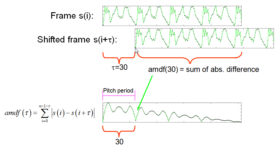
The concept of AMDF (average magnitude difference function) is very close to ACF except that it estimates the distance instead of similarity between a frame s(i), i = 0 ~ n-1, and its delayed version via the following formula: $$amdf(\tau)=\sum_{i=0}^{n-1-\tau}|s(i)-s(i+\tau)|$$

where t is the time lag in terms of sample points. The value of t that minimizes amdf(t) over a specified range is selected as the pitch period in sample points. The following figure demonstrates the operation of AMDF:

In other words, we shift the delayed version n times and compute the absolute sum of the difference in the overlapped parts to obtain n values of AMDF. A typical example of AMDF is shown below.

Example 1: frame2amdf01.mwaveFile='sunday.wav'; au=myAudioRead(waveFile); index1=9000; frameSize=512; index2=index1+frameSize-1; frame=au.signal(index1:index2); opt=frame2pdf('defaultOpt'); opt.pdf='amdf'; opt.maxShift=length(frame); opt.method=1; amdf=frame2pdf(frame, opt); subplot(3,1,1); plot(au.signal); line(index1*[1 1], [-1 1], 'color', 'r'); line(index2*[1 1], [-1 1], 'color', 'r'); subplot(3,1,2); plot(frame); subplot(3,1,3); plot(amdf);

From the above figure, it is obvious that the pitch period point should be the local minimum located at index=132. The corresponding pitch is equal to fs/(132-1) = 16000/131 = 122.14 Hz, or 46.81 semitones. This result is close but not exactly equal to the one obtained via ACF.

In order to find the pitch point automatically, we need to manipulate the AMDF curve such that its maximum corresponds to the right pitch point. This is accomplished by the following example (which is packed into a function frame2amdf4pt.m):

Example 2: frame2amdf4pt01.mwaveFile='sunday.wav'; au=myAudioRead(waveFile); index1=9000; frameSize=512; index2=index1+frameSize-1; frame=au.signal(index1:index2); opt=frame2pdf('defaultOpt'); opt.pdf='amdf'; opt.maxShift=length(frame); opt.method=1; amdf=frame2pdf(frame, opt); amdf4pt=max(amdf)-amdf-max(amdf)*linspace(0,1,length(amdf))'; amdf4pt2=amdf4pt; maxFreq=1000; amdf4pt2(1:au.fs/maxFreq)=-inf; minFreq=40; amdf4pt2(au.fs/minFreq:end)=-inf; [maxValue, maxIndex]=max(amdf4pt2); fprintf('Pitch = %f Hz = %f semitone\n', au.fs/(maxIndex-1), freq2pitch(au.fs/(maxIndex-1))); subplot(2,1,1); plot(frame, '.-'); title('Input frame'); subplot(2,1,2); xVec=1:length(amdf); plot(xVec, amdf4pt, '.-', xVec, amdf4pt2, 'm.-', maxIndex, maxValue, 'ksquare'); title(sprintf('AMDF vector (method = %d)', opt.method)); legend('Original AMDF4PT', 'Truncated AMDF4PT', 'AMDF pitch point');Pitch = 122.137405 Hz = 46.812019 semitone

Now here is an example using AMDF for pitch tracking:

Example 3: ptByAmdf01.mauFile='soo.wav'; opt=pitchTrackBasic('defaultOpt'); opt.frame2frameOpt.pdf='amdf'; showPlot=1; pitch=pitchTrackBasic(auFile, opt, showPlot); au=myAudioRead(auFile); frameSize=(opt.frameDuration*au.fs)/1000; hopSize=(opt.hopDuration*au.fs)/1000; frameRate=au.fs/hopSize; % No. of pitch points per sec pv.fs=16000; pv.nbits=16; % Specs for saving the synthesized pitch pv.signal=pv2wave(pitch, frameRate, pv.fs); % Convert pitch to wave pv.amplitudeNormalized=1; myAudioWrite(pv, 'sooPitchByAmdf.wav'); % Save the pv as a wav fileError in running ptByAmdf01! (Logged to scriptError.log)

Note that since pitchTrackBasic.m only picks the maximum during a reasonable range, so it has to invoke frame2amdf4pt.m which inverts the original AMDF, as shown in the previous example.

Just like ACF, there are several variations of AMDF, as explained next.

  1. Due to less overlap AMDF tapers off with the lag t. To avoid the tapering-off, we can normalize AMDF by dividing it by the length of the overlap: $$amdf(\tau)=\sum_{i=0}^{n-1-\tau}\frac{|s(i)-s(i+\tau)|}{n-\tau}$$ The down sides include more computation and less robustness when t is small. Here is an example.

    Example 4: frame2amdf02.mwaveFile='sunday.wav'; au=myAudioRead(waveFile); index1=9000; frameSize=512; index2=index1+frameSize-1; frame=au.signal(index1:index2); opt=frame2pdf('defaultOpt'); opt.pdf='amdf'; opt.maxShift=length(frame); opt.method=2; showPlot=1; frame2pdf(frame, opt, showPlot);

    The corresponding pitch tracking is shown next:

    Example 5: ptByamdf02.mwaveFile='soo.wav'; opt=pitchTrackBasic('defaultOpt'); opt.frame2pdfOpt.pdf='amdf'; opt.frame2pdfOpt.method=2; showPlot=1; pitch=pitchTrackBasic(waveFile, opt, showPlot);

  2. Another method to avoid AMDF's taper-off is to shift the first half of the frame only: $$amdf(\tau)=\sum_{i=0}^{n/2}|s(i)-s(i+\tau)|$$ In the following example, the length of the shifted segment is only 256, leading to an AMDF of 256 points:

    Example 6: frame2amdf03.mwaveFile='sunday.wav'; au=myAudioRead(waveFile); index1=9000; frameSize=512; index2=index1+frameSize-1; frame=au.signal(index1:index2); opt=frame2pdf('defaultOpt'); opt.pdf='amdf'; opt.maxShift=length(frame)/2; opt.method=3; showPlot=1; frame2pdf(frame, opt, showPlot);

    The corresponding pitch tracking is shown next:

    Example 7: ptByamdf03.mwaveFile='soo.wav'; opt=pitchTrackBasic('defaultOpt'); opt.frameDuration=32*2; % Duration (in ms) of a frame opt.overlapDuration=32; % Duration (in ms) of overlap opt.frame2pdfOpt.pdf='amdf'; opt.frame2pdfOpt.method=3; showPlot=1; pitch=pitchTrackBasic(waveFile, opt, showPlot);

    If the energy of the first half-frame is smaller than that of the second half-frame, it is better to flip the frame first such that a more reliable AMDF curve can be obtained.

Since the computation of AMDF does not require multiplication, it is suitable for low computing platform such as embedded systems or micro-controllers.

It is possible to combine ACF and AMDF to identify the pitch period point in a more robust manner. For instance, we can divide ACF by AMDF to obtain a curve for easy selection of the pitch point. For example:

Example 8: frame2acfOverAmdf01.mwaveFile='soo.wav'; au=myAudioRead(waveFile); frameSize=256; frameMat=enframe(au.signal, frameSize, 0); frame=frameMat(:, 292); opt=frame2pdf('defaultOpt'); opt.pdf='acfOverAmdf'; opt.maxShift=length(frame); opt.method=1; showPlot=1; acf=frame2pdf(frame, opt, showPlot);

In the above example, we have used the singing voices from Prof. Soo who was the tenor of the choir at National Taiwan University. In the selected frame, the maxima of ACF or the minima of AMDF is not very obvious. But if we divide ACF by AMDF, the maxima of the final curves are much more obvious than either ACF or AMDF alone.

In the next example, we shall use variations of ACF and AMDF for computing ACF/AMDF:

Example 9: frame2acfOverAmdf02.mwaveFile='soo.wav'; au=myAudioRead(waveFile); frameSize=256; overlap=0; frameMat=enframe(au.signal, frameSize, overlap); frame=frameMat(:, 290); subplot(4,1,1); plot(frame, '.-'); axis tight title('Input frame'); subplot(4,1,2); method=1; out=frame2acfOverAmdf(frame, frameSize, method); plot(out, '.-'); title('ACF/AMDF, method=1'); axis tight subplot(4,1,3); method=2; out=frame2acfOverAmdf(frame, frameSize, method); plot(out, '.-'); title('ACF/AMDF, method=2'); axis tight subplot(4,1,4); method=3; out=frame2acfOverAmdf(frame, frameSize/2, method); plot(out, '.-'); title('ACF/AMDF, method=3'); axis tight

In the above example, method=1 and method=2 lead to the same ACF/AMDF curve. The corresponding pitch tracking is shown next:

Example 10: ptByAcfOverAmdf01.mwaveFile='soo.wav'; opt=pitchTrackBasic('defaultOpt'); opt.frame2pitchOpt.pdf='acfOverAmdf'; opt.frame2pdfOpt.method=3; showPlot=1; pitch=pitchTrackBasic(waveFile, opt, showPlot);


Audio Signal Processing and Recognition (音訊處理與辨識)