[chinese ][english ] (請注意:中文版本並未隨英文版本同步更新! )
Linear scaling (LS for short), also known as uniform scaling or global scaling, is the most straightforward frame-based method for melody recognition. Typical linear scaling involves the following three steps:
在不切音符的情況下,最簡單的辨識方法,就是線性伸縮(Linear Scaling),流程如下:
Use interpolation to expand or compress the input pitch vector linearly. The scaling factor , defined as the length ratio between the scaled and the original vectors, could range from 0.5 to 2.0. If we take the step of 0.1 for the scaling factor, it leads to 16 expanded or compressed versions of the original pitch vector. Of course, the scaling-factor bounds ([0.5, 2.0] for instance) and the resolution (the number of scaled pitch vectors, 16 for instance) are all adjustable parameters.
Compare these 16 time-scaled versions with each song in the database. The minimum distance is then defined as the distance of the input pitch vector to a song in the database. You can simply use L1 or L2 norm to compute the distance, with appropriate processing for key transposition, to be detailed later.
For a given input pitch vector, compute the distances to all songs in the database. The song with the minimum distance is the most likely song for the input pitch vector.
使用內差法,將使用者輸入的音高向量進行線性拉長或壓縮,例如伸縮比例可以是從 0.5 到 2.0,跳距是 0.1,共生出 16 個版本。
將這16個版本和資料庫中的每一首歌曲進行比對,得到16個距離,其中的最小值,即是輸入向量和此首歌的距離。
對所有資料庫歌曲進行比對,最短距離者,即是使用者所唱的歌。
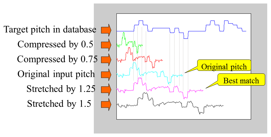
The following plot is a typical example of linear scaling, with a scaling-factor bounds of [0.5, 2] and a resolution of 5. When the scaling factor is 1.5, the minimum distance is achieved.
下面是一個線性伸縮的示意圖,共伸縮五次,當伸縮比例是 1.5 時,可以達到最佳的比對效果:
Simple as it is, in practice, we still need to consider the following detailed issues:
在實做上,還有下列細節要考慮:
Method for interpolation: Simple linear interpolation should suffice. Other advanced interpolations may be tried only if they will not make the computation prohibitive.
Distance measures: We can use L1 norm (the sum of absolute difference of elements, also known as taxicab distance or Manhattan distance) or L2 norm (square root of the sum of squared difference of elements, also known as Euclidean distance) to compute the distance.
Hint Lp norm of vectors x and y = [S |xi -yi |p ]1/p
Distance normalization: Usually we need to normalize the distance by the length of the vector to eliminate the biased introduced via expansion or compression.
Key transposition: To achieve invariance in key transposition, we need to shift the input pitch vector to achieve a minimum distance when compared to the songs in the database. For different distance measures, we have different schemes for key transposition:
For L1 norm, we can shift the input pitch vector to have the same median as that of each song in the database.
For L2 norm, we can shift the input pitch vector to have the same mean as that of each song in the database.
Rest handling: In order to preserve the timing information, we usually replace the rest with previous non-rest pitch for both input pitch vector and songs in the database. One typical example is "Row, Row, Row Your Boat" (original site , local copy ).
內差法的選用:可以使用簡單的線性內差。
距離的選擇:通常我們使用 L1 norm,也就是計算每個對應元素絕對差值的和,或是使用 L2 norm,又稱為歐基理德距離,也就是計算每個對應元素差值的平方和,再開平方,但在實做上,我們通常只在比較距離的大小,因此常常省略開平方的動作,以節省計算。
Hint Lp norm of vectors x and y = [S |xi -yi |p ]1/p
距離的正規化:我們會將總距離除以點數,得到正規化的距離,以消除因伸縮造成點數不同所帶來的影響。
音高的校正:每一個人唱歌的key不同(通常女生的key比較高,男生的key比較低),因此在進行比對之前,要先進行校正。一般而言,校正的目的是要達到兩個向量之間距離的最小值,因此對於不同的距離計算方式,我們就有不同的校正法則:
若使用 L1 norm,我們可以採用「中位數校正」,亦即將輸入向量的中位數校正成對應資料庫向量的中位數。
若使用 L2 norm,我們可以採用「平均值校正」,亦即將輸入向量的平均值校正成對應資料庫向量的平均值。
對於休止符的處理:為了保持音符的特性,我們通常會將休止符(包含使用者的輸入和資料庫的歌曲)代換成前一個音。
Characteristics of LS for melody recognition can be summarized as follows:
If the user's singing or humming is at a constant pace, LS usually gives satisfactory performance.
LS is also very efficient both in its computation and the one-shot way to handle key transposition.
線性伸縮用於旋律辨識的特性,可以說明如下:
如果使用者哼唱的歌聲不是忽快忽慢,那麼線性伸縮都可以達到不錯的辨識效果。
線性伸縮可以使用「一次到位」的音高校正,所以在計算上比較簡單。(相對而言,DTW 無法使用「一次到位」的音高校正,所以在計算上會比較繁複。)
The following example is a typical result of using LS to find the best scaling ratio of the input query:
以下是使用真實音高向量的範例:
Example 1: linScaling01.m inputPitch=[48.044247 48.917323 49.836778 50.154445 50.478049 50.807818 51.143991 51.486821 51.486821 51.486821 51.143991 50.154445 50.154445 50.154445 49.218415 51.143991 51.143991 50.807818 49.524836 49.524836 49.524836 49.524836 51.143991 51.143991 51.143991 51.486821 51.836577 50.807818 51.143991 52.558029 51.486821 51.486821 51.486821 51.143991 51.143991 51.143991 51.143991 51.143991 51.143991 51.143991 51.143991 51.143991 49.218415 50.807818 50.807818 50.154445 50.478049 48.044247 49.524836 52.193545 51.486821 51.486821 51.143991 50.807818 51.486821 51.486821 51.486821 51.486821 51.486821 55.788268 55.349958 54.922471 54.922471 55.349958 55.349958 55.349958 55.349958 55.349958 55.349958 55.349958 55.349958 53.699915 58.163541 59.213095 59.762739 59.762739 59.762739 59.762739 58.163541 57.661699 58.163541 58.680365 58.680365 58.680365 58.163541 55.788268 54.505286 55.349958 55.788268 55.788268 55.788268 54.922471 54.505286 56.237965 55.349958 55.349958 55.349958 55.349958 54.505286 54.505286 55.349958 48.917323 50.478049 50.807818 51.143991 51.143991 51.143991 50.807818 50.807818 50.478049 50.807818 51.486821 51.486821 51.486821 51.486821 51.486821 51.486821 52.558029 52.558029 52.558029 52.558029 52.193545 51.836577 52.193545 53.310858 53.310858 53.310858 52.930351 52.930351 53.310858 52.930351 52.558029 52.193545 52.930351 53.310858 52.930351 51.836577 52.558029 53.699915 52.930351 52.930351 52.558029 52.930351 52.930351 52.558029 52.558029 52.558029 53.310858 53.310858 53.310858 53.310858 52.930351 52.930351 52.930351 52.558029 52.930351 52.930351 52.930351 52.930351 52.930351 52.930351 52.930351 53.310858 53.310858 53.310858 52.193545 52.193545 52.193545 54.097918 52.930351 52.930351 52.930351 52.930351 52.930351 51.143991 51.143991 51.143991 48.917323 49.524836 49.524836 49.836778 49.524836 48.917323 49.524836 49.218415 48.330408 48.330408 48.330408 48.330408 48.330408 49.524836 49.836778 53.310858 53.310858 53.310858 52.930351 52.930351 52.930351 53.310858 52.930351 52.930351 52.558029 52.558029 51.143991 52.930351 49.218415 49.836778 50.154445 49.836778 49.524836 48.621378 48.621378 48.621378 49.836778 49.836778 49.836778 49.836778 46.680365 46.680365 46.680365 46.163541 45.661699 45.661699 45.910801 46.163541 46.163541 46.163541 46.163541 46.163541 46.163541 46.163541 46.163541 46.163541 46.163541 46.163541 46.163541 50.807818 51.486821 51.486821 51.143991];
dbPitch =[60 60 60 60 60 60 60 60 60 60 60 60 60 60 60 60 60 60 60 60 60 60 60 60 60 60 60 60 60 60 60 60 60 60 60 60 60 60 60 60 60 60 60 60 60 60 60 60 60 64 64 64 64 64 64 64 64 64 64 64 64 64 67 67 67 67 67 67 67 67 67 67 67 67 64 64 64 64 64 64 64 64 64 64 64 64 64 60 60 60 60 60 60 60 60 60 60 60 60 60 62 62 62 62 62 62 62 62 62 62 62 62 62 62 62 62 62 62 62 62 62 62 62 62 62 62 62 62 62 62 62 62 62 62 62 62 62 62 62 62 62 62 62 62 62 62 62 62 62 59 59 59 59 59 59 59 59 59 59 59 59 59 62 62 62 62 62 62 62 62 62 62 62 62 59 59 59 59 59 59 59 59 59 59 59 59 59 55 55 55 55 55 55 55 55 55 55 55 55 55 60 60 60 60 60 60 60 60 60 60 60 60 60 60 60 60 60 60 60 60 60 60 60 60 60 60 60 60 60 60 60 60 60 60 60 60 60 60 60 60 60 60 60 60 60 60 60 60 60 64 64 64 64 64 64 64 64 64 64 64 64 64 67 67 67 67 67 67 67 67 67 67 67 67 64 64 64 64 64 64 64 64 64 64 64 64 64 60 60 60 60 60 60 60 60 60 60 60 60 60 67 67 67 67 67 67 67 67 67 67 67 67 65 65 65 65 65 65 65 65 65 65 65 65 65 64 64 64 64 64 64 64 64 64 64 64 64 62 62 62 62 62 62 62 62 62 62 62 62 62 60 60 60 60 60 60 60 60 60 60 60 60 60];
resolution=21;
sfBounds=[0.5, 1.5]; % Scaling-factor bounds
distanceType=1; % L1-norm
[minDist1, scaledPitch, allDist]=linScaling(inputPitch, dbPitch, sfBounds(1), sfBounds(2), resolution, distanceType);
axisLimit=[0 370 45 70];
subplot(3,1,1);
plot(1:length(dbPitch), dbPitch, '.-', 1:length(inputPitch), inputPitch, '.-');
title('Database and input pitch vectors'); ylabel('Semitones');
legend('Database pitch', 'Input pitch', 'location', 'SouthEast');
axis(axisLimit);
subplot(3,1,2);
plot(1:length(dbPitch), dbPitch, '.-', 1:length(scaledPitch), scaledPitch, '.-');
legend('Database pitch', 'Scaled pitch', 'location', 'SouthEast');
title('Database and scaled pitch vectors'); ylabel('Semitones');
axis(axisLimit);
subplot(3,1,3);
ratio=linspace(sfBounds(1), sfBounds(2), resolution);
plot(ratio, allDist, '.-');
xlabel('Scaling factor'); ylabel('Distance'); title(sprintf('Normalized distance of L_%d norm', distanceType));
LS is rather robust to the use of different distance metrics, as shown in the following example where L1 and L2 norms are used to obtain the same result.
下列範例採用兩種距離函數 L1 -norm 和 L2 -norm 來進行 LS,所得到的結果很接近:
Example 2: linScaling02.m inputPitch=[48.044247 48.917323 49.836778 50.154445 50.478049 50.807818 51.143991 51.486821 51.486821 51.486821 51.143991 50.154445 50.154445 50.154445 49.218415 51.143991 51.143991 50.807818 49.524836 49.524836 49.524836 49.524836 51.143991 51.143991 51.143991 51.486821 51.836577 50.807818 51.143991 52.558029 51.486821 51.486821 51.486821 51.143991 51.143991 51.143991 51.143991 51.143991 51.143991 51.143991 51.143991 51.143991 49.218415 50.807818 50.807818 50.154445 50.478049 48.044247 49.524836 52.193545 51.486821 51.486821 51.143991 50.807818 51.486821 51.486821 51.486821 51.486821 51.486821 55.788268 55.349958 54.922471 54.922471 55.349958 55.349958 55.349958 55.349958 55.349958 55.349958 55.349958 55.349958 53.699915 58.163541 59.213095 59.762739 59.762739 59.762739 59.762739 58.163541 57.661699 58.163541 58.680365 58.680365 58.680365 58.163541 55.788268 54.505286 55.349958 55.788268 55.788268 55.788268 54.922471 54.505286 56.237965 55.349958 55.349958 55.349958 55.349958 54.505286 54.505286 55.349958 48.917323 50.478049 50.807818 51.143991 51.143991 51.143991 50.807818 50.807818 50.478049 50.807818 51.486821 51.486821 51.486821 51.486821 51.486821 51.486821 52.558029 52.558029 52.558029 52.558029 52.193545 51.836577 52.193545 53.310858 53.310858 53.310858 52.930351 52.930351 53.310858 52.930351 52.558029 52.193545 52.930351 53.310858 52.930351 51.836577 52.558029 53.699915 52.930351 52.930351 52.558029 52.930351 52.930351 52.558029 52.558029 52.558029 53.310858 53.310858 53.310858 53.310858 52.930351 52.930351 52.930351 52.558029 52.930351 52.930351 52.930351 52.930351 52.930351 52.930351 52.930351 53.310858 53.310858 53.310858 52.193545 52.193545 52.193545 54.097918 52.930351 52.930351 52.930351 52.930351 52.930351 51.143991 51.143991 51.143991 48.917323 49.524836 49.524836 49.836778 49.524836 48.917323 49.524836 49.218415 48.330408 48.330408 48.330408 48.330408 48.330408 49.524836 49.836778 53.310858 53.310858 53.310858 52.930351 52.930351 52.930351 53.310858 52.930351 52.930351 52.558029 52.558029 51.143991 52.930351 49.218415 49.836778 50.154445 49.836778 49.524836 48.621378 48.621378 48.621378 49.836778 49.836778 49.836778 49.836778 46.680365 46.680365 46.680365 46.163541 45.661699 45.661699 45.910801 46.163541 46.163541 46.163541 46.163541 46.163541 46.163541 46.163541 46.163541 46.163541 46.163541 46.163541 46.163541 50.807818 51.486821 51.486821 51.143991];
dbPitch =[60 60 60 60 60 60 60 60 60 60 60 60 60 60 60 60 60 60 60 60 60 60 60 60 60 60 60 60 60 60 60 60 60 60 60 60 60 60 60 60 60 60 60 60 60 60 60 60 60 64 64 64 64 64 64 64 64 64 64 64 64 64 67 67 67 67 67 67 67 67 67 67 67 67 64 64 64 64 64 64 64 64 64 64 64 64 64 60 60 60 60 60 60 60 60 60 60 60 60 60 62 62 62 62 62 62 62 62 62 62 62 62 62 62 62 62 62 62 62 62 62 62 62 62 62 62 62 62 62 62 62 62 62 62 62 62 62 62 62 62 62 62 62 62 62 62 62 62 62 59 59 59 59 59 59 59 59 59 59 59 59 59 62 62 62 62 62 62 62 62 62 62 62 62 59 59 59 59 59 59 59 59 59 59 59 59 59 55 55 55 55 55 55 55 55 55 55 55 55 55 60 60 60 60 60 60 60 60 60 60 60 60 60 60 60 60 60 60 60 60 60 60 60 60 60 60 60 60 60 60 60 60 60 60 60 60 60 60 60 60 60 60 60 60 60 60 60 60 60 64 64 64 64 64 64 64 64 64 64 64 64 64 67 67 67 67 67 67 67 67 67 67 67 67 64 64 64 64 64 64 64 64 64 64 64 64 64 60 60 60 60 60 60 60 60 60 60 60 60 60 67 67 67 67 67 67 67 67 67 67 67 67 65 65 65 65 65 65 65 65 65 65 65 65 65 64 64 64 64 64 64 64 64 64 64 64 64 62 62 62 62 62 62 62 62 62 62 62 62 62 60 60 60 60 60 60 60 60 60 60 60 60 60];
resolution=21;
sfBounds=[0.5, 1.5]; % Scaling-factor bounds
distanceType=1; % L1-norm
[minDist1, scaledPitch1, allDist1]=linScaling(inputPitch, dbPitch, sfBounds(1), sfBounds(2), resolution, distanceType);
distanceType=2; % L2-norm
[minDist1, scaledPitch2, allDist2]=linScaling(inputPitch, dbPitch, sfBounds(1), sfBounds(2), resolution, distanceType);
allDist2=sqrt(allDist2); % To reduce computation, the L2-distance returned by linScalingMex is actually the square distance, so we need to take the square root.
axisLimit=[0 370 45 70];
subplot(3,1,1);
plot(1:length(dbPitch), dbPitch, '.-', 1:length(inputPitch), inputPitch, '.-');
title('Database and input pitch vectors'); ylabel('Semitones');
legend('Database pitch', 'Input pitch', 'location', 'SouthEast');
axis(axisLimit);
subplot(3,1,2);
plot(1:length(dbPitch), dbPitch, '.-', 1:length(scaledPitch1), scaledPitch1, '.-', 1:length(scaledPitch2), scaledPitch2, '.-');
legend('Database pitch', 'Scaled pitch via L_1 norm', 'Scaled pitch via L_2 norm', 'location', 'SouthEast');
title('Database and scaled pitch vectors'); ylabel('Semitones');
axis(axisLimit);
subplot(3,1,3);
ratio=linspace(sfBounds(1), sfBounds(2), resolution);
plot(ratio, allDist1, '.-', ratio, allDist2, '.-');
xlabel('Scaling factor'); ylabel('Distances'); title('Normalized distances via L_1 & L_2 norm');
legend('L_1 norm', 'L_2 norm', 'location', 'SouthEast');
Hint Note that in order to save computation, linScalingMex uses the square of L2 norm instead of L2 norm literally. Therefore we need to do square root in order to get the correct distance based on L2 norm.
Hint 請注意,為了節省計算,上述範例中 linScalingMex 的距離計算,是使用 L2 norm 的平方,而不是使用 L2 norm。所以最後在畫圖前,我們還要進行開平方,以便得到正確的 L2 norm。
Audio Signal Processing and Recognition (音訊處理與辨識)