Tutorial on Voiced Sound Detection for Polyphonic Audio Music
This tutorial describes the basics of voiced sound detection (VSD). In particular, the audio files used for our analysis are singing/humming recordings with human labeled frame-based pitch as the groundtruth. Here the voiced sound refer to the frames the recordings which have pitch. In other words, this is a binary classification problem given the mixture of vocal and background music. We shall try to tackle this problem with several common methods.
Contents
Preprocessing
Before we start, let's add necessary toolboxes to the search path of MATLAB:
addpath d:/users/jang/matlab/toolbox/utility
addpath d:/users/jang/matlab/toolbox/sap
addpath d:/users/jang/matlab/toolbox/machineLearning
All the above toolboxes can be downloaded from the author's toolbox page. Make sure you are using the latest toolboxes to work with this script.
For compatibility, here we list the platform and MATLAB version that we used to run this script:
fprintf('Platform: %s\n', computer);
fprintf('MATLAB version: %s\n', version);
fprintf('Script starts at %s\n', char(datetime));
scriptStartTime=tic;	% Timing for the whole script
Platform: PCWIN64
MATLAB version: 9.6.0.1214997 (R2019a) Update 6
Script starts at 18-Jan-2020 18:51:25
For this script, most of the modifiable options are set in vsdOptSet.m:
type vsdOptSet
function vsdOpt=vsdOptSet
% vsdOptSet: Set options for VSD (voiced sound detection) for audio music
%
%	Usage:
%		vsdOpt=vsdOptSet;
%
%	Description:
%		vsdOpt=vsdOptSet returns the default options for voiced sound detection.
%
%	Example:
%		vsdOpt=vsdOptSet

%	Category: Options for voiced sound detection
%	Roger Jang, 20130114

%% === Basic options for VSD
vsdOpt.fs=16000;
vsdOpt.frameSize=640;
vsdOpt.overlap=320;
vsdOpt.gaussianNum=4;	% No. of Gaussians for each class
vsdOpt.outputName={'s/u', 'voiced'};	% s/u: silence & unoviced
%% === Function for feature extraction and plotting
vsdOpt.feaExtractFcn=@vsdFeaExtract;
vsdOpt.hmmPlotFcn=@vsdHmmPlot;
%% === Folder for audio files (downloaded from "http://mirlab.org/dataSet/public")
vsdOpt.audioDir='D:\dataSet\public\MIR-1K\Wavfile';		% Folder holding audio files
vsdOpt.pitchDir='D:\dataSet\public\MIR-1K\PitchLabel';	% Folder of pitch files
You can change options in this file to try other settings for VSD. In particular, the following changes are mandatory if you want to run this script on your machine:
- Make "vsdOpt.audioDir" point to the audio folder of the MIR-1K corpus.
- Make "vsdOpt.pitchDir" point to the pitch folder of the MIR-1K corpus.
The MIR-1K corpus is available at here.
Dataset collection
We can now read all the audio files (that have been manually labeled with frame-based pitch) to perform feature extraction. Note that: * The result is stored in a big structure varaible auSet for further analysis. * We also save auSet to vsdAuSet.mat so that we don't need to do it again next time. * If the program finds vsdAuSet.mat, it'll load the file directly to restore auSet. * If you prefer to redo the feature extraction, you need to delete "vsdAuSet.mat" in advance.
Here it goes:
vsdOpt=vsdOptSet;
auFileNum=20;		% Use only this number of audio files
if ~exist('vsdAuSet.mat', 'file')
	myTic=tic;
	fprintf('Collecting audio files and their features from "%s"...\n', vsdOpt.audioDir);
	auSet=recursiveFileList(vsdOpt.audioDir, 'wav');	% Collect all wav files
	auSet=auSet(1:auFileNum);
	auSet=auSetFeaExtract(auSet, vsdOpt);
	fprintf('Time for feature extraction over %d files = %g sec\n', length(auSet), toc(myTic));
	fprintf('Saving auSet to vsdAuSet.mat...\n');
	save vsdAuSet auSet
else
	fprintf('Loading auSet from vsdAuSet.mat...\n');
	load vsdAuSet.mat
end
Loading auSet from vsdAuSet.mat...
Now we can create a variable ds for data visualization and classification:
ds.input=[auSet.feature];
ds.output=[auSet.tOutput];
ds.inputName=auSet(1).other.inputName;
ds.outputName=vsdOpt.outputName;
We can obtain the feature dimensions and data count:
[dim, count]=size(ds.input);
fprintf('Feature dimensions = %d, data count = %d\n', dim, count);
Feature dimensions = 13, data count = 8494
Since the dataset is big, we reduce the dataset for easy plotting:
downSampleRatio=2;
ds.input=ds.input(:, 1:downSampleRatio:end);
ds.output=ds.output(:, 1:downSampleRatio:end);
fprintf('Data count = %d after 1/%d down sampling.\n', size(ds.input, 2), downSampleRatio);
Data count = 4247 after 1/2 down sampling.
Data analysis and visualization
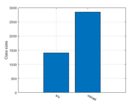
Display data sizes for each class:
[classSize, classLabel]=dsClassSize(ds, 1);
13 features
4247 instances
2 classes
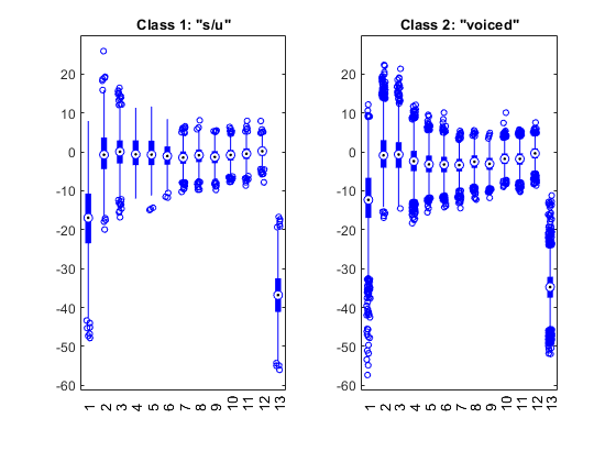
Display feature distribution for each class:
figure; dsBoxPlot(ds);
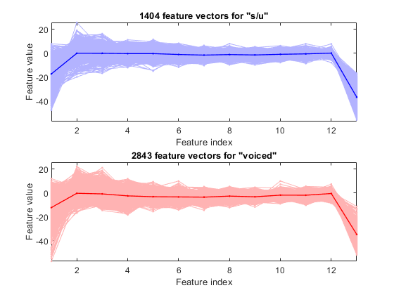
Plot the feature vectors within each class:
figure; dsFeaVecPlot(ds);
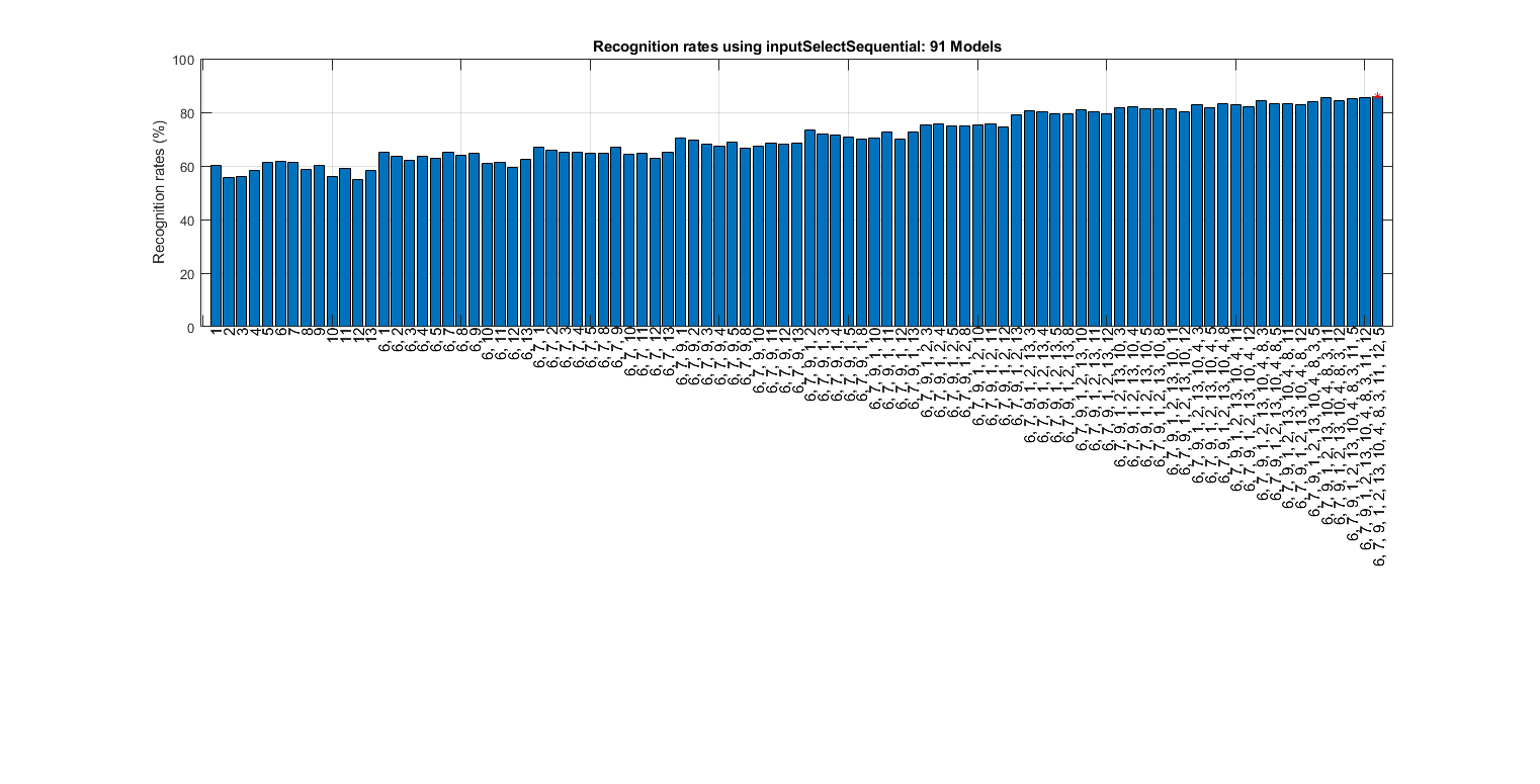
Input selection
We can select more important inputs based on leave-one-out (LOO) criterion of KNNC:
myTic=tic;
figure; bestInputIndex=inputSelectSequential(ds); figEnlarge;
fprintf('time=%g sec\n', toc(myTic));
Construct 91 "knnc" models, each with up to 13 inputs selected from all 13 inputs...

Selecting input 1:
Model 1/91: selected={1} => Recog. rate = 60.3%
Model 2/91: selected={2} => Recog. rate = 55.5%
Model 3/91: selected={3} => Recog. rate = 55.9%
Model 4/91: selected={4} => Recog. rate = 58.5%
Model 5/91: selected={5} => Recog. rate = 61.5%
Model 6/91: selected={6} => Recog. rate = 61.5%
Model 7/91: selected={7} => Recog. rate = 61.4%
Model 8/91: selected={8} => Recog. rate = 58.6%
Model 9/91: selected={9} => Recog. rate = 60.1%
Model 10/91: selected={10} => Recog. rate = 56.1%
Model 11/91: selected={11} => Recog. rate = 59.1%
Model 12/91: selected={12} => Recog. rate = 54.9%
Model 13/91: selected={13} => Recog. rate = 58.3%
Currently selected inputs: 6 => Recog. rate = 61.5%

Selecting input 2:
Model 14/91: selected={6, 1} => Recog. rate = 65.2%
Model 15/91: selected={6, 2} => Recog. rate = 63.7%
Model 16/91: selected={6, 3} => Recog. rate = 62.0%
Model 17/91: selected={6, 4} => Recog. rate = 63.5%
Model 18/91: selected={6, 5} => Recog. rate = 62.8%
Model 19/91: selected={6, 7} => Recog. rate = 65.2%
Model 20/91: selected={6, 8} => Recog. rate = 64.0%
Model 21/91: selected={6, 9} => Recog. rate = 64.7%
Model 22/91: selected={6, 10} => Recog. rate = 60.8%
Model 23/91: selected={6, 11} => Recog. rate = 61.2%
Model 24/91: selected={6, 12} => Recog. rate = 59.5%
Model 25/91: selected={6, 13} => Recog. rate = 62.6%
Currently selected inputs: 6, 7 => Recog. rate = 65.2%

Selecting input 3:
Model 26/91: selected={6, 7, 1} => Recog. rate = 66.8%
Model 27/91: selected={6, 7, 2} => Recog. rate = 66.0%
Model 28/91: selected={6, 7, 3} => Recog. rate = 64.9%
Model 29/91: selected={6, 7, 4} => Recog. rate = 64.9%
Model 30/91: selected={6, 7, 5} => Recog. rate = 64.7%
Model 31/91: selected={6, 7, 8} => Recog. rate = 64.8%
Model 32/91: selected={6, 7, 9} => Recog. rate = 67.1%
Model 33/91: selected={6, 7, 10} => Recog. rate = 64.5%
Model 34/91: selected={6, 7, 11} => Recog. rate = 64.8%
Model 35/91: selected={6, 7, 12} => Recog. rate = 63.0%
Model 36/91: selected={6, 7, 13} => Recog. rate = 64.9%
Currently selected inputs: 6, 7, 9 => Recog. rate = 67.1%

Selecting input 4:
Model 37/91: selected={6, 7, 9, 1} => Recog. rate = 70.4%
Model 38/91: selected={6, 7, 9, 2} => Recog. rate = 69.5%
Model 39/91: selected={6, 7, 9, 3} => Recog. rate = 68.1%
Model 40/91: selected={6, 7, 9, 4} => Recog. rate = 67.5%
Model 41/91: selected={6, 7, 9, 5} => Recog. rate = 68.8%
Model 42/91: selected={6, 7, 9, 8} => Recog. rate = 66.7%
Model 43/91: selected={6, 7, 9, 10} => Recog. rate = 67.3%
Model 44/91: selected={6, 7, 9, 11} => Recog. rate = 68.3%
Model 45/91: selected={6, 7, 9, 12} => Recog. rate = 68.0%
Model 46/91: selected={6, 7, 9, 13} => Recog. rate = 68.6%
Currently selected inputs: 6, 7, 9, 1 => Recog. rate = 70.4%

Selecting input 5:
Model 47/91: selected={6, 7, 9, 1, 2} => Recog. rate = 73.3%
Model 48/91: selected={6, 7, 9, 1, 3} => Recog. rate = 71.8%
Model 49/91: selected={6, 7, 9, 1, 4} => Recog. rate = 71.4%
Model 50/91: selected={6, 7, 9, 1, 5} => Recog. rate = 70.8%
Model 51/91: selected={6, 7, 9, 1, 8} => Recog. rate = 70.1%
Model 52/91: selected={6, 7, 9, 1, 10} => Recog. rate = 70.5%
Model 53/91: selected={6, 7, 9, 1, 11} => Recog. rate = 72.8%
Model 54/91: selected={6, 7, 9, 1, 12} => Recog. rate = 70.0%
Model 55/91: selected={6, 7, 9, 1, 13} => Recog. rate = 72.5%
Currently selected inputs: 6, 7, 9, 1, 2 => Recog. rate = 73.3%

Selecting input 6:
Model 56/91: selected={6, 7, 9, 1, 2, 3} => Recog. rate = 75.4%
Model 57/91: selected={6, 7, 9, 1, 2, 4} => Recog. rate = 75.6%
Model 58/91: selected={6, 7, 9, 1, 2, 5} => Recog. rate = 75.0%
Model 59/91: selected={6, 7, 9, 1, 2, 8} => Recog. rate = 75.1%
Model 60/91: selected={6, 7, 9, 1, 2, 10} => Recog. rate = 75.2%
Model 61/91: selected={6, 7, 9, 1, 2, 11} => Recog. rate = 75.5%
Model 62/91: selected={6, 7, 9, 1, 2, 12} => Recog. rate = 74.5%
Model 63/91: selected={6, 7, 9, 1, 2, 13} => Recog. rate = 78.9%
Currently selected inputs: 6, 7, 9, 1, 2, 13 => Recog. rate = 78.9%

Selecting input 7:
Model 64/91: selected={6, 7, 9, 1, 2, 13, 3} => Recog. rate = 80.7%
Model 65/91: selected={6, 7, 9, 1, 2, 13, 4} => Recog. rate = 80.3%
Model 66/91: selected={6, 7, 9, 1, 2, 13, 5} => Recog. rate = 79.3%
Model 67/91: selected={6, 7, 9, 1, 2, 13, 8} => Recog. rate = 79.6%
Model 68/91: selected={6, 7, 9, 1, 2, 13, 10} => Recog. rate = 80.9%
Model 69/91: selected={6, 7, 9, 1, 2, 13, 11} => Recog. rate = 80.1%
Model 70/91: selected={6, 7, 9, 1, 2, 13, 12} => Recog. rate = 79.3%
Currently selected inputs: 6, 7, 9, 1, 2, 13, 10 => Recog. rate = 80.9%

Selecting input 8:
Model 71/91: selected={6, 7, 9, 1, 2, 13, 10, 3} => Recog. rate = 81.8%
Model 72/91: selected={6, 7, 9, 1, 2, 13, 10, 4} => Recog. rate = 82.1%
Model 73/91: selected={6, 7, 9, 1, 2, 13, 10, 5} => Recog. rate = 81.3%
Model 74/91: selected={6, 7, 9, 1, 2, 13, 10, 8} => Recog. rate = 81.4%
Model 75/91: selected={6, 7, 9, 1, 2, 13, 10, 11} => Recog. rate = 81.3%
Model 76/91: selected={6, 7, 9, 1, 2, 13, 10, 12} => Recog. rate = 80.3%
Currently selected inputs: 6, 7, 9, 1, 2, 13, 10, 4 => Recog. rate = 82.1%

Selecting input 9:
Model 77/91: selected={6, 7, 9, 1, 2, 13, 10, 4, 3} => Recog. rate = 82.8%
Model 78/91: selected={6, 7, 9, 1, 2, 13, 10, 4, 5} => Recog. rate = 81.8%
Model 79/91: selected={6, 7, 9, 1, 2, 13, 10, 4, 8} => Recog. rate = 83.0%
Model 80/91: selected={6, 7, 9, 1, 2, 13, 10, 4, 11} => Recog. rate = 82.6%
Model 81/91: selected={6, 7, 9, 1, 2, 13, 10, 4, 12} => Recog. rate = 81.9%
Currently selected inputs: 6, 7, 9, 1, 2, 13, 10, 4, 8 => Recog. rate = 83.0%

Selecting input 10:
Model 82/91: selected={6, 7, 9, 1, 2, 13, 10, 4, 8, 3} => Recog. rate = 84.2%
Model 83/91: selected={6, 7, 9, 1, 2, 13, 10, 4, 8, 5} => Recog. rate = 83.1%
Model 84/91: selected={6, 7, 9, 1, 2, 13, 10, 4, 8, 11} => Recog. rate = 83.1%
Model 85/91: selected={6, 7, 9, 1, 2, 13, 10, 4, 8, 12} => Recog. rate = 82.7%
Currently selected inputs: 6, 7, 9, 1, 2, 13, 10, 4, 8, 3 => Recog. rate = 84.2%

Selecting input 11:
Model 86/91: selected={6, 7, 9, 1, 2, 13, 10, 4, 8, 3, 5} => Recog. rate = 83.9%
Model 87/91: selected={6, 7, 9, 1, 2, 13, 10, 4, 8, 3, 11} => Recog. rate = 85.3%
Model 88/91: selected={6, 7, 9, 1, 2, 13, 10, 4, 8, 3, 12} => Recog. rate = 84.2%
Currently selected inputs: 6, 7, 9, 1, 2, 13, 10, 4, 8, 3, 11 => Recog. rate = 85.3%

Selecting input 12:
Model 89/91: selected={6, 7, 9, 1, 2, 13, 10, 4, 8, 3, 11, 5} => Recog. rate = 85.1%
Model 90/91: selected={6, 7, 9, 1, 2, 13, 10, 4, 8, 3, 11, 12} => Recog. rate = 85.6%
Currently selected inputs: 6, 7, 9, 1, 2, 13, 10, 4, 8, 3, 11, 12 => Recog. rate = 85.6%

Selecting input 13:
Model 91/91: selected={6, 7, 9, 1, 2, 13, 10, 4, 8, 3, 11, 12, 5} => Recog. rate = 85.8%
Currently selected inputs: 6, 7, 9, 1, 2, 13, 10, 4, 8, 3, 11, 12, 5 => Recog. rate = 85.8%

Overall maximal recognition rate = 85.8%.
Selected 13 inputs (out of 13): 6, 7, 9, 1, 2, 13, 10, 4, 8, 3, 11, 12, 5
time=17.0366 sec
Input transformation
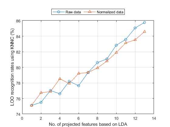
We can also perform LDA and evaluation of its performance based on LOO criterion. To get a quick result, here we find the transformation matrix using all data points and then evaluate KNNC performance based on LOO. This is only an approximate result and it tends to be on the optimistic side:
myTic=tic;
ds2=ds; ds2.input=inputNormalize(ds2.input);	% input normalization
opt=ldaPerfViaKnncLoo('defaultOpt');
opt.mode='approximate';
recogRate1=ldaPerfViaKnncLoo(ds, opt);
recogRate2=ldaPerfViaKnncLoo(ds2, opt);
figure; plot(1:length(recogRate1), 100*recogRate1, 'o-', 1:length(recogRate2), 100*recogRate2, '^-'); grid on
legend('Raw data', 'Normalized data', 'location', 'northOutside', 'orientation', 'horizontal');
xlabel('No. of projected features based on LDA');
ylabel('LOO recognition rates using KNNC (%)');
fprintf('time=%g sec\n', toc(myTic));
time=6.27666 sec
It would be too time consuming to perform the LDA evaluation of exact LOO. But if you do want to try it, uncomment the following code:
%myTic=tic;
%ds2=ds; ds2.input=inputNormalize(ds2.input);	% input normalization
%opt=ldaPerfViaKnncLoo('defaultOpt');
%opt.mode='exact';
%recogRate1=ldaPerfViaKnncLoo(ds, opt);
%recogRate2=ldaPerfViaKnncLoo(ds2, opt);
%figure; plot(1:length(recogRate1), 100*recogRate1, 'o-', 1:length(recogRate2), 100*recogRate2, '^-'); grid on
%legend('Raw data', 'Normalized data', 'location', 'northOutside', 'orientation', 'horizontal');
%xlabel('No. of projected features based on LDA');
%ylabel('LOO recognition rates using KNNC (%)');
%fprintf('time=%g sec\n', toc(myTic));
HMM training
Using the collected auSet, we can start HMM training for voiced sound detection:
myTic=tic;
[vsdHmmModel, rr]=hmmTrain4audio(auSet, vsdOpt, 1); figEnlarge;
fprintf('Time for HMM training=%g sec\n', toc(myTic));
Time for HMM training=6.91248 sec
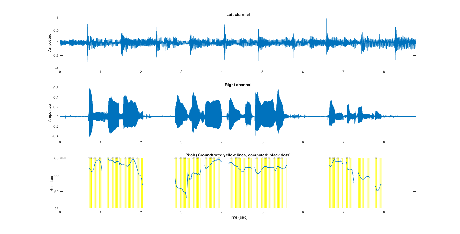
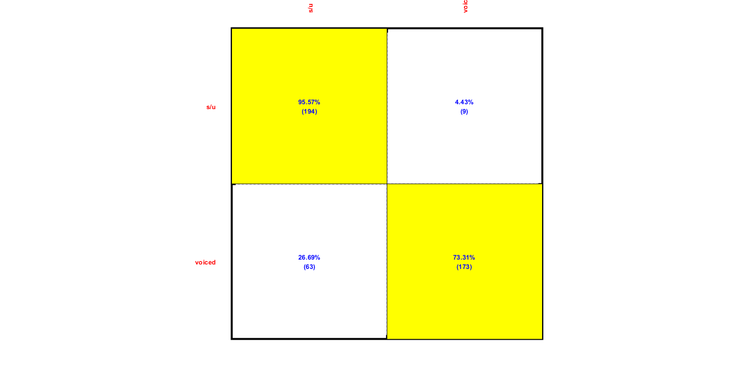
HMM test
After the training, we can test the HMM using a single audio file:
myTic=tic;
auFile=auSet(1).path;
au=myAudioRead(auFile);
au=vsdOpt.feaExtractFcn(au, vsdOpt, 1);	% Attach feature and tOutput
wObj=hmmEval4audio(au, vsdOpt, vsdHmmModel, 1); figEnlarge;
fprintf('time=%g sec\n', toc(myTic));
Warning: data dim is larger than 2. The plot is based on the first 2 dimensions
Accuracy=83.5991%
time=1.80526 sec
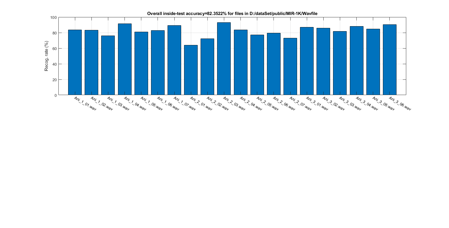
Performance evaluation of HMM via LOO
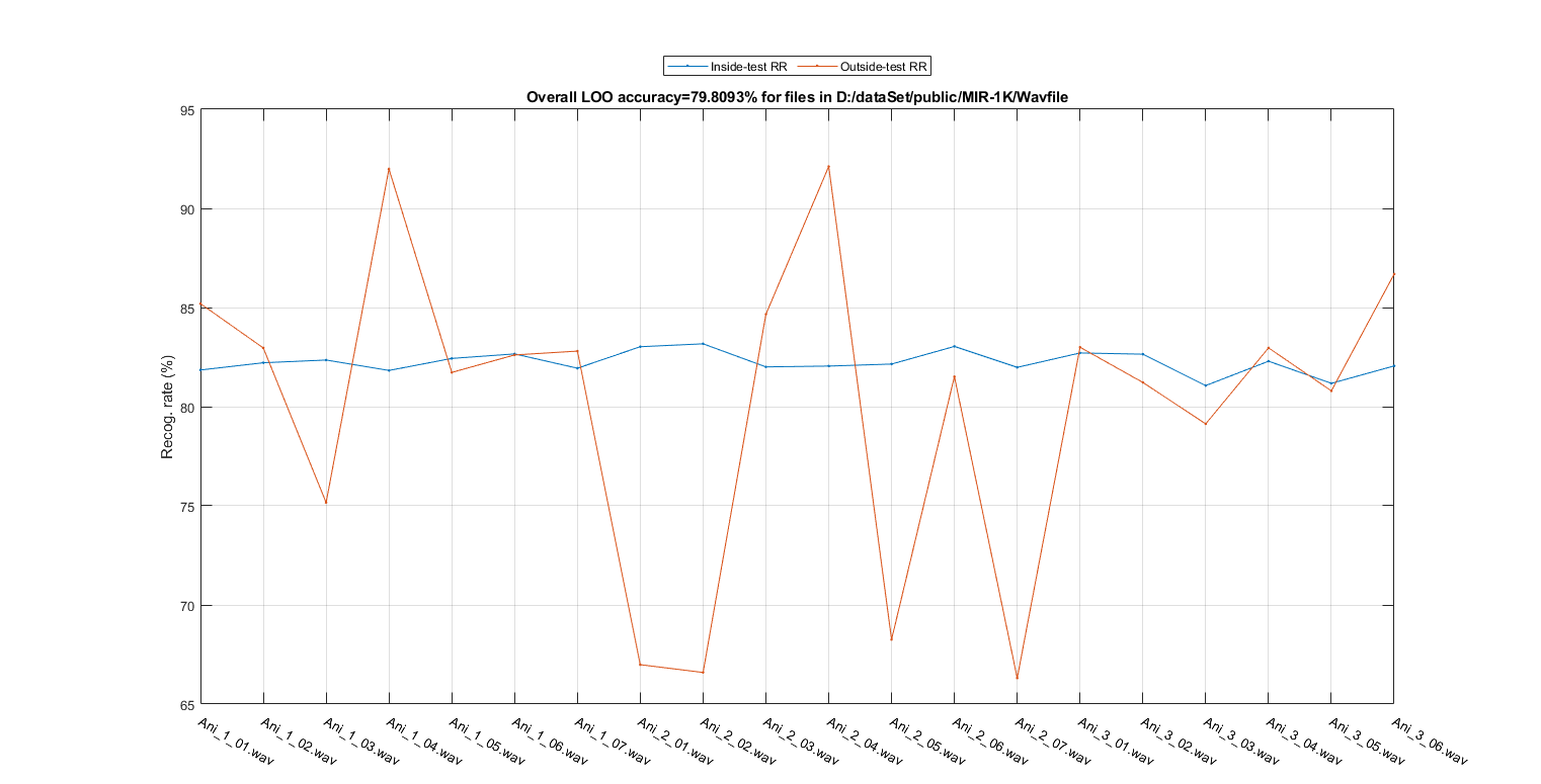
To evaluate the performance more objectively, we can test the LOO accuracy by using "leave-one-file-out". (Note that it's very time consuming.)
myTic=tic;
showPlot=1;
[outsideRr, cvData]=hmmPerfLoo4audio(auSet, vsdOpt, showPlot); figEnlarge;
fprintf('time=%g sec\n', toc(myTic));
1/20: file=D:\dataSet\public\MIR-1K\Wavfile/Ani_1_01.wav
	outsideRr=85.1936%, time=6.38415 sec
2/20: file=D:\dataSet\public\MIR-1K\Wavfile/Ani_1_02.wav
	outsideRr=82.9615%, time=6.33041 sec
3/20: file=D:\dataSet\public\MIR-1K\Wavfile/Ani_1_03.wav
	outsideRr=75.1634%, time=6.36853 sec
4/20: file=D:\dataSet\public\MIR-1K\Wavfile/Ani_1_04.wav
	outsideRr=91.9872%, time=6.37268 sec
5/20: file=D:\dataSet\public\MIR-1K\Wavfile/Ani_1_05.wav
	outsideRr=81.7284%, time=6.51878 sec
6/20: file=D:\dataSet\public\MIR-1K\Wavfile/Ani_1_06.wav
	outsideRr=82.6087%, time=6.39278 sec
7/20: file=D:\dataSet\public\MIR-1K\Wavfile/Ani_1_07.wav
	outsideRr=82.8025%, time=6.18789 sec
8/20: file=D:\dataSet\public\MIR-1K\Wavfile/Ani_2_01.wav
	outsideRr=66.9872%, time=5.76201 sec
9/20: file=D:\dataSet\public\MIR-1K\Wavfile/Ani_2_02.wav
	outsideRr=66.5944%, time=6.07305 sec
10/20: file=D:\dataSet\public\MIR-1K\Wavfile/Ani_2_03.wav
	outsideRr=84.6591%, time=6.41975 sec
11/20: file=D:\dataSet\public\MIR-1K\Wavfile/Ani_2_04.wav
	outsideRr=92.1136%, time=6.40226 sec
12/20: file=D:\dataSet\public\MIR-1K\Wavfile/Ani_2_05.wav
	outsideRr=68.254%, time=6.22957 sec
13/20: file=D:\dataSet\public\MIR-1K\Wavfile/Ani_2_06.wav
	outsideRr=81.5157%, time=6.28366 sec
14/20: file=D:\dataSet\public\MIR-1K\Wavfile/Ani_2_07.wav
	outsideRr=66.3102%, time=6.06415 sec
15/20: file=D:\dataSet\public\MIR-1K\Wavfile/Ani_3_01.wav
	outsideRr=82.9966%, time=6.18037 sec
16/20: file=D:\dataSet\public\MIR-1K\Wavfile/Ani_3_02.wav
	outsideRr=81.2207%, time=5.65851 sec
17/20: file=D:\dataSet\public\MIR-1K\Wavfile/Ani_3_03.wav
	outsideRr=79.1319%, time=5.42375 sec
18/20: file=D:\dataSet\public\MIR-1K\Wavfile/Ani_3_04.wav
	outsideRr=82.9653%, time=6.42115 sec
19/20: file=D:\dataSet\public\MIR-1K\Wavfile/Ani_3_05.wav
	outsideRr=80.7958%, time=5.48512 sec
20/20: file=D:\dataSet\public\MIR-1K\Wavfile/Ani_3_06.wav
	outsideRr=86.6883%, time=5.52775 sec
Overall LOO accuracy=79.8093%
time=122.65 sec
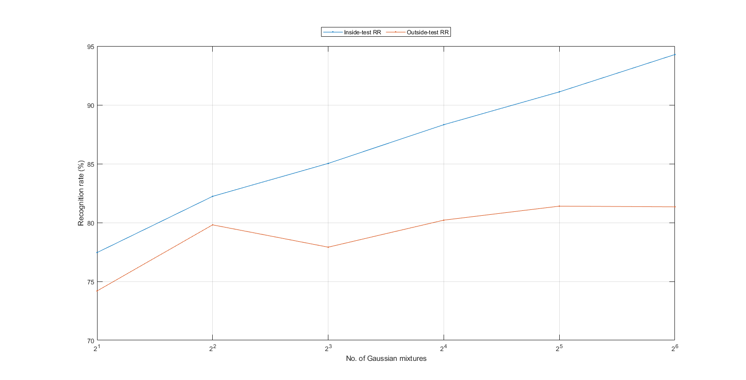
We can then detect the best number of Gaussian components in each state of the HMM using such leave-one-file-out cross validation. This part is also time consuming:
myTic=tic;
maxExponent=6;
insideRr=zeros(1, maxExponent);
for i=1:maxExponent
	vsdOpt.gaussianNum=2^i;
	fprintf('%d/%d: No. of Gaussian component=%d, ', i, maxExponent, vsdOpt.gaussianNum);
	[outsideRr(i), cvData]=hmmPerfLoo4audio(auSet, vsdOpt);
	insideRr(i)=mean([cvData.insideRr]);
	fprintf('insideRR=%g%%, outsideRr=%g%%\n', insideRr(i)*100, outsideRr(i)*100);
end
plot(1:maxExponent, insideRr*100, '.-', 1:maxExponent, outsideRr*100, '.-'); grid on; figEnlarge;
set(gca, 'xTick', 1:maxExponent);
label=get(gca, 'xticklabel');
for i=1:length(label), label{i}=sprintf('2^%s', label{i}); end;
set(gca, 'xticklabel', label);
legend('Inside-test RR', 'Outside-test RR', 'location', 'northOutside', 'orientation', 'horizontal');
xlabel('No. of Gaussian mixtures');
ylabel('Recognition rate (%)');
fprintf('time=%g sec\n', toc(myTic));
1/6: No. of Gaussian component=2, insideRR=77.4539%, outsideRr=74.1935%
2/6: No. of Gaussian component=4, insideRR=82.2318%, outsideRr=79.8093%
3/6: No. of Gaussian component=8, insideRR=85.0299%, outsideRr=77.9138%
4/6: No. of Gaussian component=16, insideRR=88.3201%, outsideRr=80.2096%
5/6: No. of Gaussian component=32, insideRR=91.1104%, outsideRr=81.3986%
6/6: No. of Gaussian component=64, insideRR=94.2833%, outsideRr=81.3398%
time=3058.52 sec
Summary
This is a brief tutorial on using HMM for voiced sound detection for polyphonic audio music. There are several directions for further improvement:
- Explore other preprocessing, such as HPSS.
- Investigate new features for VSD.
- Change the configuration of the GMM used in HMM.
- Use of other classifiers for VSD.
Appendix
List of functions and datasets used in this script
Date and time when finishing this script:
fprintf('Date & time: %s\n', char(datetime));
Date & time: 18-Jan-2020 19:45:16
Overall elapsed time:
toc(scriptStartTime)
Elapsed time is 3231.415313 seconds.
Date and time when finishing this script:
fprintf('Date & time: %s\n', char(datetime));
Date & time: 18-Jan-2020 19:45:16
If you are interested in the original MATLAB code for this page, you can type "grabcode(URL)" under MATLAB, where URL is the web address of this page.