Tutorial on Vibrato Detection (by Roger Jang)
This tutorial explains how to use HMM (Hidden Markov Models) for VD (vibrato detection) in human's singing voice. Here the human's singing voice is referred to pure vocals without any accompaniment. Such vibrato detection can be used in singing voice scoring, especially in karaoke machines.
Contents
Preprocessing
Before we start, let's add necessary toolboxes to the search path of MATLAB:
addpath d:/users/jang/matlab/toolbox/utility
addpath d:/users/jang/matlab/toolbox/sap
addpath d:/users/jang/matlab/toolbox/machineLearning
All the above toolboxes can be downloaded from the author's toolbox page. Make sure you are using the latest toolboxes to work with this script.
For compatibility, here we list the platform and MATLAB version that we used to run this script:
fprintf('Platform: %s\n', computer);
fprintf('MATLAB version: %s\n', version);
fprintf('Date & time: %s\n', char(datetime));
scriptStartTime=tic;	% Timing for the whole script
Platform: PCWIN64
MATLAB version: 9.6.0.1214997 (R2019a) Update 6
Date & time: 18-Jan-2020 19:46:57
Most of the modifiable options for this vibrato detection task are set in vdOptSet.m:
type vdOptSet
function vdOpt=vdOptSet
% vdOptSet: Set options for VD (vibrato detection)
%
%	Usage:
%		vdOpt=vdOptSet;
%
%	Description:
%		vdOpt=vdOptSet returns the default options for vibrato detection.
%
%	Example:
%		vdOpt=vdOptSet

%	Category: Options for vibrato detection
%	Roger Jang, 20130114

%% === Function for feature extraction and plotting
vdOpt.feaExtractFcn=@vdFeaExtractFromFile;
%vdOpt.feaExtractFcn=@vibratoFeaExtract;
vdOpt.hmmPlotFcn=@vdHmmPlot;
%% === Folder for wave files
vdOpt.audioDir='D:\dataset\vibrato\TeresaTeng\waveAndPitch';
%% === Parameters for VD
vdOpt.frameSize=512;
vdOpt.overlap=0;
vdOpt.pfType=1;		% For pitch tracking, 0 for AMDF, 1 for ACF
vdOpt.sFrameSizeInSec=0.3;	% Super frame size
vdOpt.sOverlapInSec=0;		% Super overlap
vdOpt.featureName={'aPitch', 'bPitch', 'distPitch', 'aVol', 'bVol', 'distVol'};
%vdOpt.featureName={'aPitch', 'bPitch', 'distPitch'};
vdOpt.outputName={'nonvibrato', 'vibrato'};
vdOpt.classNum=length(vdOpt.outputName);
vdOpt.gaussianNum=3;	% No. of Gaussians for each class
If you want to run this script, you need to change vdOpt.audioDir such that it points to a folder of sound files containing singing voices with vibrato. The dataset used in the script can be downloaded from <http://mirlab.org/dataset/public>.
Dataset collection
First of all, we can collect all the sound files once they are downloaded. We can use the commmand "mmDataCollect" to collect all the file information:
vdOpt=vdOptSet;
opt=mmDataCollect('defaultOpt');
opt.extName='wav';
auSet=mmDataCollect(vdOpt.audioDir, opt, 1);
Collecting 12 files with extension "wav" from "D:\dataset\vibrato\TeresaTeng\waveAndPitch"...
We can now read all the wave files (that have been labeled with vibrato segments), perform feature extraction, and store the result in a big structure varaible auSet:
myTic=tic;
auSet=auSetFeaExtract(auSet, vdOpt, 1);
fprintf('Saving vdAuSet.mat...\n');
save vdAuSet auSet
fprintf('time=%g sec\n', toc(myTic));
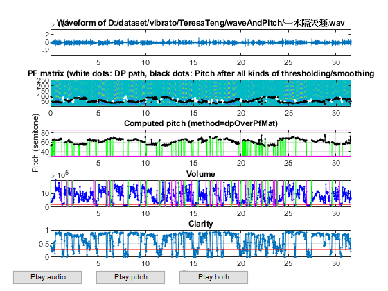
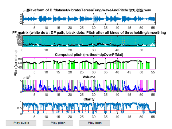
1/12: file=D:\dataset\vibrato\TeresaTeng\waveAndPitch/一水隔天涯.wav, duration=31.6071 sec, time=8.7052 sec
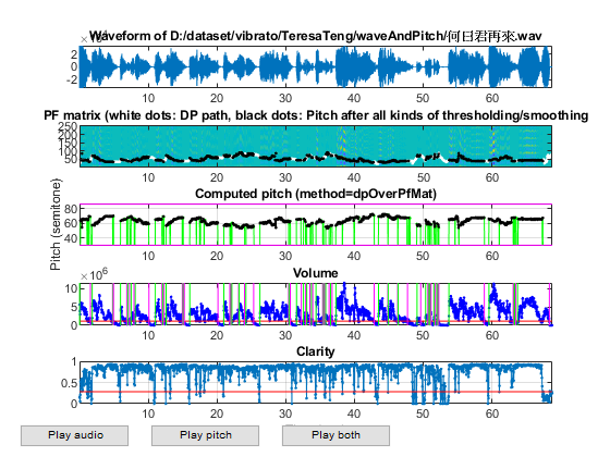
2/12: file=D:\dataset\vibrato\TeresaTeng\waveAndPitch/何日君再來.wav, duration=68.7801 sec, time=13.9216 sec
3/12: file=D:\dataset\vibrato\TeresaTeng\waveAndPitch/你怎麼說.wav, duration=56.1401 sec, time=8.82078 sec
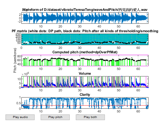
4/12: file=D:\dataset\vibrato\TeresaTeng\waveAndPitch/再見我的愛人.wav, duration=65.3401 sec, time=10.7131 sec
5/12: file=D:\dataset\vibrato\TeresaTeng\waveAndPitch/夜來香.wav, duration=61.0001 sec, time=11.2794 sec
6/12: file=D:\dataset\vibrato\TeresaTeng\waveAndPitch/小媳婦回娘家.wav, duration=61.6901 sec, time=13.3599 sec
7/12: file=D:\dataset\vibrato\TeresaTeng\waveAndPitch/帝女花.wav, duration=76.8601 sec, time=10.1244 sec
8/12: file=D:\dataset\vibrato\TeresaTeng\waveAndPitch/梅花.wav, duration=242.012 sec, time=35.8829 sec
9/12: file=D:\dataset\vibrato\TeresaTeng\waveAndPitch/獨上西樓.wav, duration=52.9102 sec, time=9.65708 sec
10/12: file=D:\dataset\vibrato\TeresaTeng\waveAndPitch/相似淚.wav, duration=91.3201 sec, time=19.8694 sec
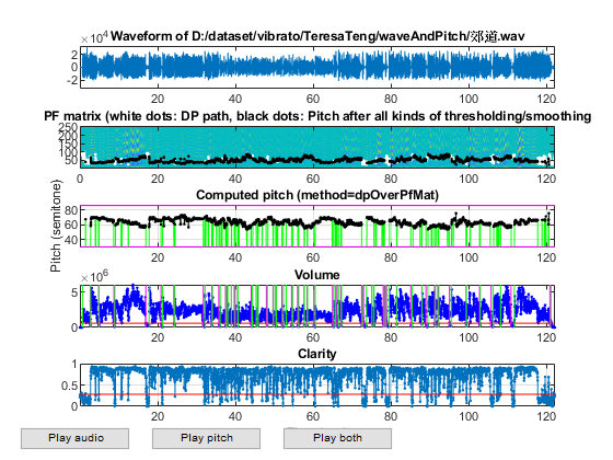
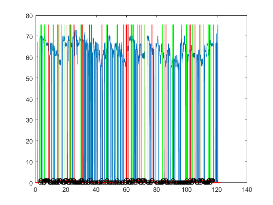
11/12: file=D:\dataset\vibrato\TeresaTeng\waveAndPitch/郊道.wav, duration=122.16 sec, time=30.5902 sec
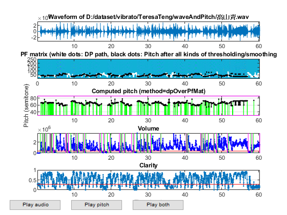
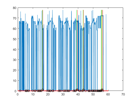
12/12: file=D:\dataset\vibrato\TeresaTeng\waveAndPitch/高山青.wav, duration=60.2945 sec, time=10.1485 sec
Total time=230.726 sec
Saving vdAuSet.mat...
time=230.777 sec
We can also create DS for all kinds of data visualization tools:
feature=[auSet.feature];
output=[auSet.tOutput];
temp=[auSet.other]; invalidIndex=[temp.invalidIndex];
feature(:, invalidIndex)=[];
output(:, invalidIndex)=[];
DS.input=feature;
DS.output=output;
DS.inputName=vdOpt.featureName;
DS.outputName=vdOpt.outputName;
DS2=DS; DS2.input=inputNormalize(DS2.input);	% input normalization
Data analysis and visualization
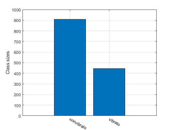
Display data count for each class:
[classSize, classLabel]=dsClassSize(DS, 1);
6 features
1353 instances
2 classes
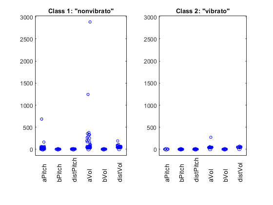
Display feature distribution among different classes:
figure; dsBoxPlot(DS);
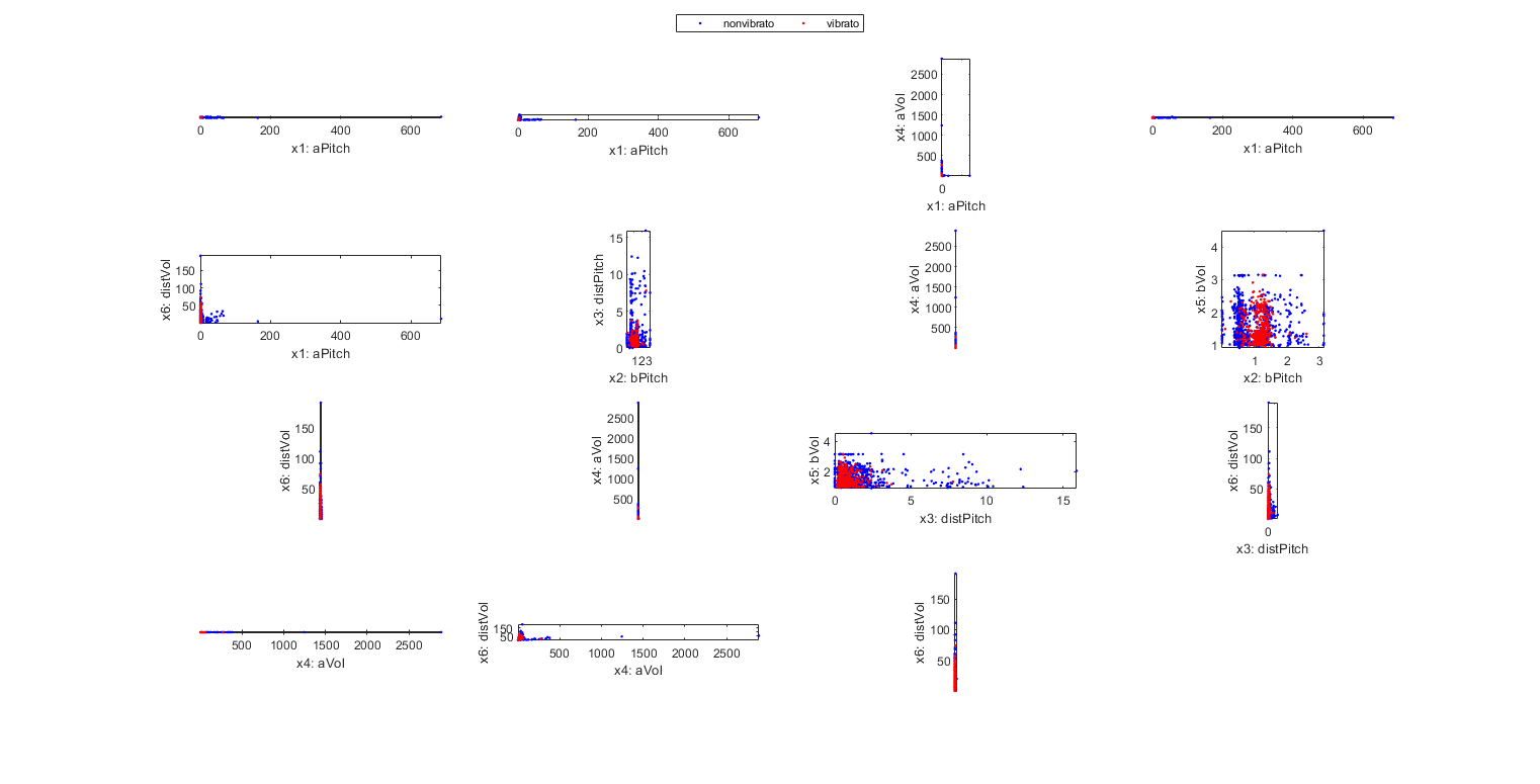
Scatter plot of the original DS to 2D:
figure; dsProjPlot2(DS); figEnlarge;
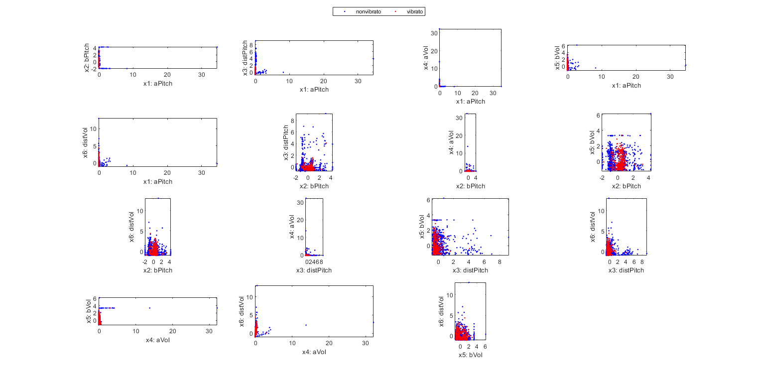
Scatter plot of the input-normalized DS to 2D:
figure; dsProjPlot2(DS2); figEnlarge;
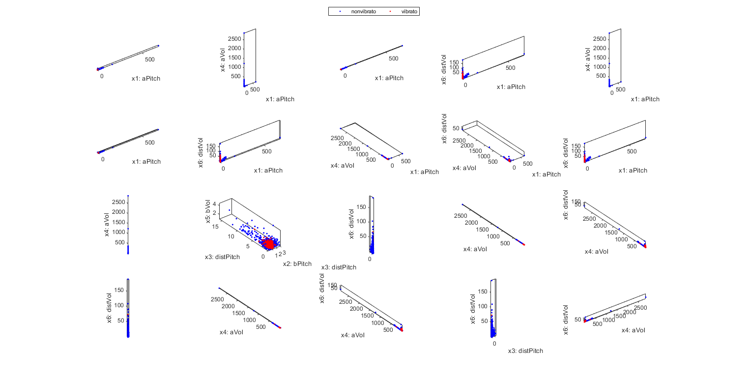
Scatter plot of the original DS to 3D:
figure; dsProjPlot3(DS); figEnlarge;
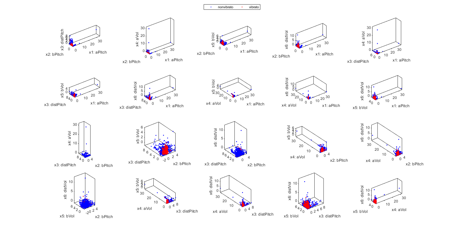
Scatter plot of the input-normalized DS to 3D:
figure; dsProjPlot3(DS2); figEnlarge;
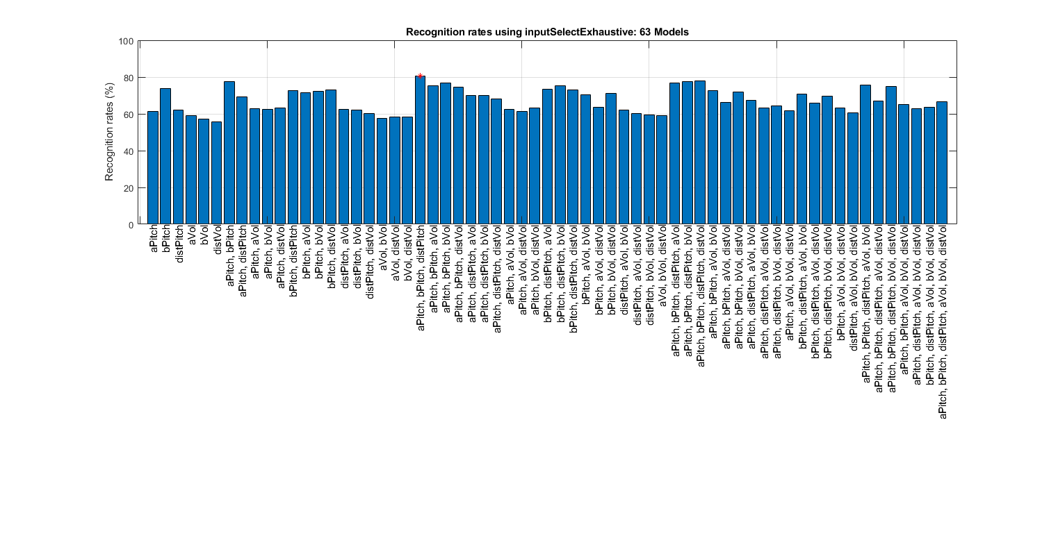
Input selection based on KNNC, using the original dataset:
myTic=tic;
inputSelectExhaustive(DS); figEnlarge;
fprintf('time=%g sec\n', toc(myTic));
Construct 63 knnc models, each with up to 6 inputs selected from 6 candidates...
modelIndex 1/63: selected={aPitch} => Recog. rate = 61.197339%
modelIndex 2/63: selected={bPitch} => Recog. rate = 73.909830%
modelIndex 3/63: selected={distPitch} => Recog. rate = 61.936438%
modelIndex 4/63: selected={aVol} => Recog. rate = 58.906135%
modelIndex 5/63: selected={bVol} => Recog. rate = 57.354028%
modelIndex 6/63: selected={distVol} => Recog. rate = 55.728012%
modelIndex 7/63: selected={aPitch, bPitch} => Recog. rate = 77.383592%
modelIndex 8/63: selected={aPitch, distPitch} => Recog. rate = 69.253511%
modelIndex 9/63: selected={aPitch, aVol} => Recog. rate = 62.897265%
modelIndex 10/63: selected={aPitch, bVol} => Recog. rate = 62.379897%
modelIndex 11/63: selected={aPitch, distVol} => Recog. rate = 63.192905%
modelIndex 12/63: selected={bPitch, distPitch} => Recog. rate = 72.727273%
modelIndex 13/63: selected={bPitch, aVol} => Recog. rate = 71.470806%
modelIndex 14/63: selected={bPitch, bVol} => Recog. rate = 72.283814%
modelIndex 15/63: selected={bPitch, distVol} => Recog. rate = 73.096822%
modelIndex 16/63: selected={distPitch, aVol} => Recog. rate = 62.305987%
modelIndex 17/63: selected={distPitch, bVol} => Recog. rate = 62.084257%
modelIndex 18/63: selected={distPitch, distVol} => Recog. rate = 60.014782%
modelIndex 19/63: selected={aVol, bVol} => Recog. rate = 57.427938%
modelIndex 20/63: selected={aVol, distVol} => Recog. rate = 58.388766%
modelIndex 21/63: selected={bVol, distVol} => Recog. rate = 58.388766%
modelIndex 22/63: selected={aPitch, bPitch, distPitch} => Recog. rate = 80.709534%
modelIndex 23/63: selected={aPitch, bPitch, aVol} => Recog. rate = 75.314117%
modelIndex 24/63: selected={aPitch, bPitch, bVol} => Recog. rate = 76.718404%
modelIndex 25/63: selected={aPitch, bPitch, distVol} => Recog. rate = 74.575018%
modelIndex 26/63: selected={aPitch, distPitch, aVol} => Recog. rate = 69.918699%
modelIndex 27/63: selected={aPitch, distPitch, bVol} => Recog. rate = 69.844789%
modelIndex 28/63: selected={aPitch, distPitch, distVol} => Recog. rate = 67.997044%
modelIndex 29/63: selected={aPitch, aVol, bVol} => Recog. rate = 62.379897%
modelIndex 30/63: selected={aPitch, aVol, distVol} => Recog. rate = 61.419069%
modelIndex 31/63: selected={aPitch, bVol, distVol} => Recog. rate = 63.045085%
modelIndex 32/63: selected={bPitch, distPitch, aVol} => Recog. rate = 73.392461%
modelIndex 33/63: selected={bPitch, distPitch, bVol} => Recog. rate = 75.314117%
modelIndex 34/63: selected={bPitch, distPitch, distVol} => Recog. rate = 72.949002%
modelIndex 35/63: selected={bPitch, aVol, bVol} => Recog. rate = 70.509978%
modelIndex 36/63: selected={bPitch, aVol, distVol} => Recog. rate = 63.710273%
modelIndex 37/63: selected={bPitch, bVol, distVol} => Recog. rate = 70.953437%
modelIndex 38/63: selected={distPitch, aVol, bVol} => Recog. rate = 62.010347%
modelIndex 39/63: selected={distPitch, aVol, distVol} => Recog. rate = 60.310421%
modelIndex 40/63: selected={distPitch, bVol, distVol} => Recog. rate = 59.571323%
modelIndex 41/63: selected={aVol, bVol, distVol} => Recog. rate = 58.906135%
modelIndex 42/63: selected={aPitch, bPitch, distPitch, aVol} => Recog. rate = 76.792313%
modelIndex 43/63: selected={aPitch, bPitch, distPitch, bVol} => Recog. rate = 77.383592%
modelIndex 44/63: selected={aPitch, bPitch, distPitch, distVol} => Recog. rate = 77.974871%
modelIndex 45/63: selected={aPitch, bPitch, aVol, bVol} => Recog. rate = 72.653363%
modelIndex 46/63: selected={aPitch, bPitch, aVol, distVol} => Recog. rate = 66.149298%
modelIndex 47/63: selected={aPitch, bPitch, bVol, distVol} => Recog. rate = 71.766445%
modelIndex 48/63: selected={aPitch, distPitch, aVol, bVol} => Recog. rate = 67.405765%
modelIndex 49/63: selected={aPitch, distPitch, aVol, distVol} => Recog. rate = 63.192905%
modelIndex 50/63: selected={aPitch, distPitch, bVol, distVol} => Recog. rate = 64.153732%
modelIndex 51/63: selected={aPitch, aVol, bVol, distVol} => Recog. rate = 61.566888%
modelIndex 52/63: selected={bPitch, distPitch, aVol, bVol} => Recog. rate = 70.583888%
modelIndex 53/63: selected={bPitch, distPitch, aVol, distVol} => Recog. rate = 65.705839%
modelIndex 54/63: selected={bPitch, distPitch, bVol, distVol} => Recog. rate = 69.770880%
modelIndex 55/63: selected={bPitch, aVol, bVol, distVol} => Recog. rate = 63.045085%
modelIndex 56/63: selected={distPitch, aVol, bVol, distVol} => Recog. rate = 60.458241%
modelIndex 57/63: selected={aPitch, bPitch, distPitch, aVol, bVol} => Recog. rate = 75.535846%
modelIndex 58/63: selected={aPitch, bPitch, distPitch, aVol, distVol} => Recog. rate = 67.110126%
modelIndex 59/63: selected={aPitch, bPitch, distPitch, bVol, distVol} => Recog. rate = 75.092387%
modelIndex 60/63: selected={aPitch, bPitch, aVol, bVol, distVol} => Recog. rate = 64.966741%
modelIndex 61/63: selected={aPitch, distPitch, aVol, bVol, distVol} => Recog. rate = 62.675536%
modelIndex 62/63: selected={bPitch, distPitch, aVol, bVol, distVol} => Recog. rate = 63.414634%
modelIndex 63/63: selected={aPitch, bPitch, distPitch, aVol, bVol, distVol} => Recog. rate = 66.592757%

Overall max recognition rate = 80.7%.
Selected 3 inputs (out of 6): aPitch, bPitch, distPitch
time=1.97777 sec
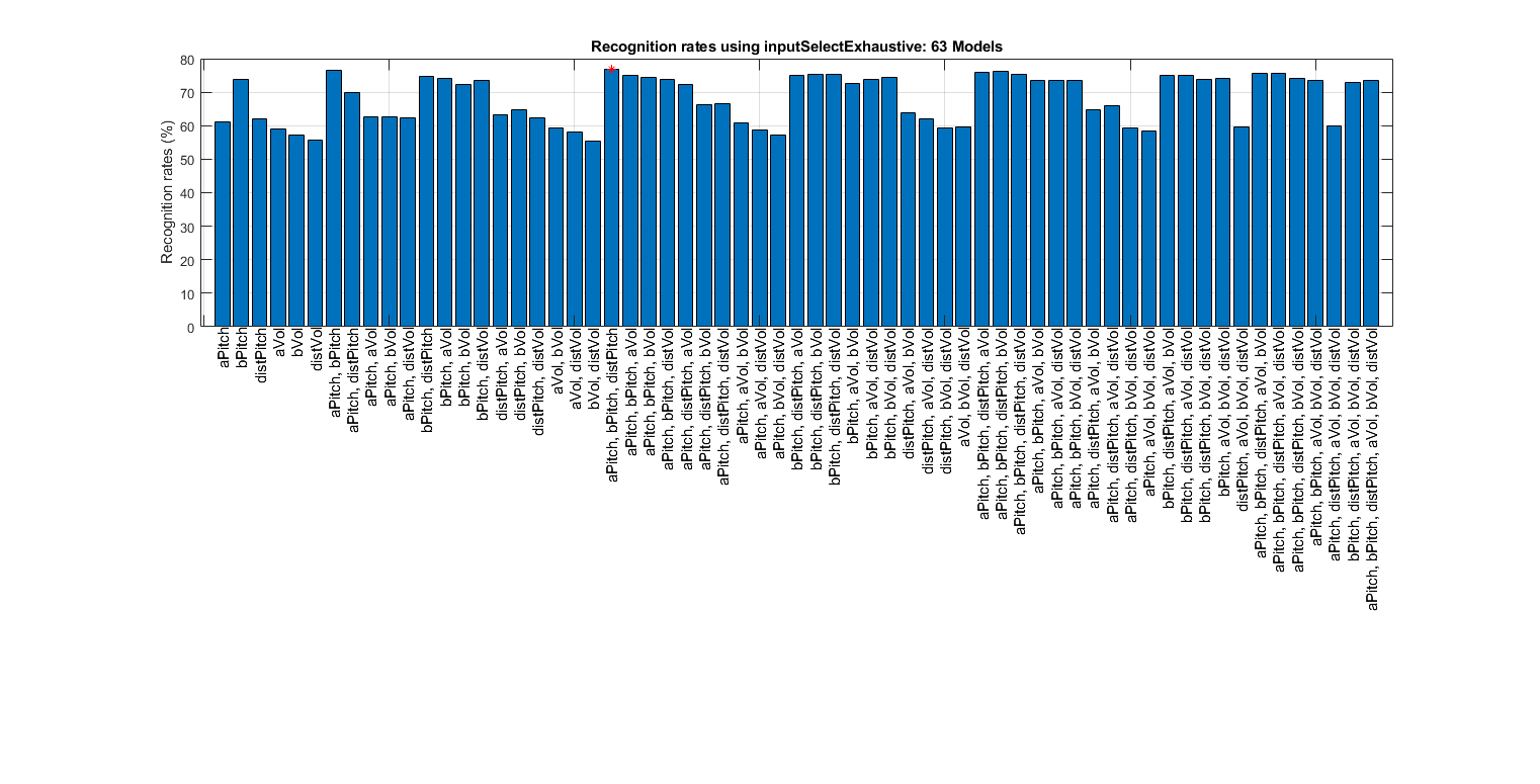
Input selection based on KNNC, using the input-normalizd dataset:
clf;
myTic=tic;
inputSelectExhaustive(DS2); figEnlarge;
fprintf('time=%g sec\n', toc(myTic));
Construct 63 knnc models, each with up to 6 inputs selected from 6 candidates...
modelIndex 1/63: selected={aPitch} => Recog. rate = 61.197339%
modelIndex 2/63: selected={bPitch} => Recog. rate = 73.909830%
modelIndex 3/63: selected={distPitch} => Recog. rate = 61.936438%
modelIndex 4/63: selected={aVol} => Recog. rate = 58.906135%
modelIndex 5/63: selected={bVol} => Recog. rate = 57.354028%
modelIndex 6/63: selected={distVol} => Recog. rate = 55.728012%
modelIndex 7/63: selected={aPitch, bPitch} => Recog. rate = 76.496674%
modelIndex 8/63: selected={aPitch, distPitch} => Recog. rate = 69.992609%
modelIndex 9/63: selected={aPitch, aVol} => Recog. rate = 62.601626%
modelIndex 10/63: selected={aPitch, bVol} => Recog. rate = 62.601626%
modelIndex 11/63: selected={aPitch, distVol} => Recog. rate = 62.232077%
modelIndex 12/63: selected={bPitch, distPitch} => Recog. rate = 74.722838%
modelIndex 13/63: selected={bPitch, aVol} => Recog. rate = 74.131559%
modelIndex 14/63: selected={bPitch, bVol} => Recog. rate = 72.283814%
modelIndex 15/63: selected={bPitch, distVol} => Recog. rate = 73.614191%
modelIndex 16/63: selected={distPitch, aVol} => Recog. rate = 63.340724%
modelIndex 17/63: selected={distPitch, bVol} => Recog. rate = 64.818921%
modelIndex 18/63: selected={distPitch, distVol} => Recog. rate = 62.232077%
modelIndex 19/63: selected={aVol, bVol} => Recog. rate = 59.423503%
modelIndex 20/63: selected={aVol, distVol} => Recog. rate = 58.240946%
modelIndex 21/63: selected={bVol, distVol} => Recog. rate = 55.432373%
modelIndex 22/63: selected={aPitch, bPitch, distPitch} => Recog. rate = 76.940133%
modelIndex 23/63: selected={aPitch, bPitch, aVol} => Recog. rate = 75.018477%
modelIndex 24/63: selected={aPitch, bPitch, bVol} => Recog. rate = 74.279379%
modelIndex 25/63: selected={aPitch, bPitch, distVol} => Recog. rate = 73.835920%
modelIndex 26/63: selected={aPitch, distPitch, aVol} => Recog. rate = 72.283814%
modelIndex 27/63: selected={aPitch, distPitch, bVol} => Recog. rate = 66.371027%
modelIndex 28/63: selected={aPitch, distPitch, distVol} => Recog. rate = 66.592757%
modelIndex 29/63: selected={aPitch, aVol, bVol} => Recog. rate = 60.975610%
modelIndex 30/63: selected={aPitch, aVol, distVol} => Recog. rate = 58.610495%
modelIndex 31/63: selected={aPitch, bVol, distVol} => Recog. rate = 57.058389%
modelIndex 32/63: selected={bPitch, distPitch, aVol} => Recog. rate = 74.870658%
modelIndex 33/63: selected={bPitch, distPitch, bVol} => Recog. rate = 75.388027%
modelIndex 34/63: selected={bPitch, distPitch, distVol} => Recog. rate = 75.388027%
modelIndex 35/63: selected={bPitch, aVol, bVol} => Recog. rate = 72.579453%
modelIndex 36/63: selected={bPitch, aVol, distVol} => Recog. rate = 73.835920%
modelIndex 37/63: selected={bPitch, bVol, distVol} => Recog. rate = 74.427199%
modelIndex 38/63: selected={distPitch, aVol, bVol} => Recog. rate = 63.858093%
modelIndex 39/63: selected={distPitch, aVol, distVol} => Recog. rate = 62.084257%
modelIndex 40/63: selected={distPitch, bVol, distVol} => Recog. rate = 59.349593%
modelIndex 41/63: selected={aVol, bVol, distVol} => Recog. rate = 59.719143%
modelIndex 42/63: selected={aPitch, bPitch, distPitch, aVol} => Recog. rate = 75.979305%
modelIndex 43/63: selected={aPitch, bPitch, distPitch, bVol} => Recog. rate = 76.127125%
modelIndex 44/63: selected={aPitch, bPitch, distPitch, distVol} => Recog. rate = 75.314117%
modelIndex 45/63: selected={aPitch, bPitch, aVol, bVol} => Recog. rate = 73.466371%
modelIndex 46/63: selected={aPitch, bPitch, aVol, distVol} => Recog. rate = 73.466371%
modelIndex 47/63: selected={aPitch, bPitch, bVol, distVol} => Recog. rate = 73.614191%
modelIndex 48/63: selected={aPitch, distPitch, aVol, bVol} => Recog. rate = 64.671101%
modelIndex 49/63: selected={aPitch, distPitch, aVol, distVol} => Recog. rate = 65.853659%
modelIndex 50/63: selected={aPitch, distPitch, bVol, distVol} => Recog. rate = 59.349593%
modelIndex 51/63: selected={aPitch, aVol, bVol, distVol} => Recog. rate = 58.388766%
modelIndex 52/63: selected={bPitch, distPitch, aVol, bVol} => Recog. rate = 75.018477%
modelIndex 53/63: selected={bPitch, distPitch, aVol, distVol} => Recog. rate = 75.018477%
modelIndex 54/63: selected={bPitch, distPitch, bVol, distVol} => Recog. rate = 73.835920%
modelIndex 55/63: selected={bPitch, aVol, bVol, distVol} => Recog. rate = 74.057650%
modelIndex 56/63: selected={distPitch, aVol, bVol, distVol} => Recog. rate = 59.497413%
modelIndex 57/63: selected={aPitch, bPitch, distPitch, aVol, bVol} => Recog. rate = 75.683666%
modelIndex 58/63: selected={aPitch, bPitch, distPitch, aVol, distVol} => Recog. rate = 75.535846%
modelIndex 59/63: selected={aPitch, bPitch, distPitch, bVol, distVol} => Recog. rate = 74.205469%
modelIndex 60/63: selected={aPitch, bPitch, aVol, bVol, distVol} => Recog. rate = 73.614191%
modelIndex 61/63: selected={aPitch, distPitch, aVol, bVol, distVol} => Recog. rate = 59.940872%
modelIndex 62/63: selected={bPitch, distPitch, aVol, bVol, distVol} => Recog. rate = 73.022912%
modelIndex 63/63: selected={aPitch, bPitch, distPitch, aVol, bVol, distVol} => Recog. rate = 73.614191%

Overall max recognition rate = 76.9%.
Selected 3 inputs (out of 6): aPitch, bPitch, distPitch
time=1.68137 sec
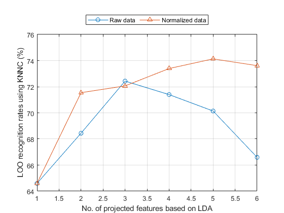
LDA evaluation of approximate LOO
figure;
myTic=tic;
opt=ldaPerfViaKnncLoo('defaultOpt');
opt.mode='approximate';
recogRate1=ldaPerfViaKnncLoo(DS, opt);
recogRate2=ldaPerfViaKnncLoo(DS2, opt);
featureNum=size(DS.input, 1);
plot(1:featureNum, 100*recogRate1, 'o-', 1:featureNum, 100*recogRate2, '^-'); grid on
legend('Raw data', 'Normalized data', 'location', 'northOutside', 'orientation', 'horizontal');
xlabel('No. of projected features based on LDA');
ylabel('LOO recognition rates using KNNC (%)');
fprintf('time=%g sec\n', toc(myTic));
time=0.413403 sec
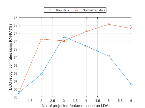
LDA evaluation of exact LOO
figure
myTic=tic;
opt=ldaPerfViaKnncLoo('defaultOpt');
opt.mode='exact';
recogRate1=ldaPerfViaKnncLoo(DS, opt);
recogRate2=ldaPerfViaKnncLoo(DS2, opt);
[featureNum, dataNum] = size(DS.input);
plot(1:featureNum, 100*recogRate1, 'o-', 1:featureNum, 100*recogRate2, '^-'); grid on
legend('Raw data', 'Normalized data', 'location', 'northOutside', 'orientation', 'horizontal');
xlabel('No. of projected features based on LDA');
ylabel('LOO recognition rates using KNNC (%)');
fprintf('time=%g sec\n', toc(myTic));
time=10.695 sec
HMM training
Using the collected auSet, we can start HMM training for vibrato detection:
figure;
myTic=tic;
vdHmmModel=hmmTrain4audio(auSet, vdOpt, 1);
fprintf('time=%g sec\n', toc(myTic));
time=0.463051 sec
HMM test
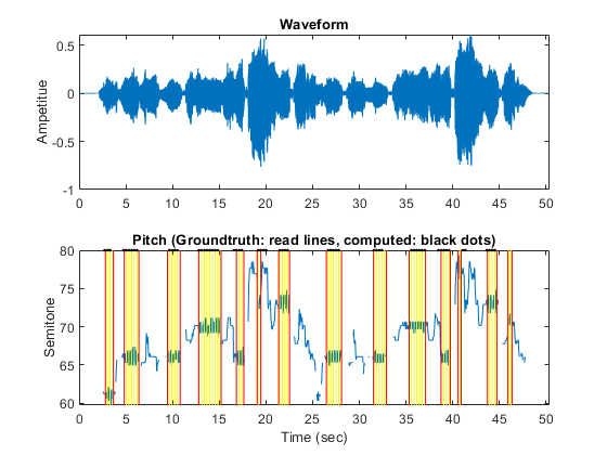
After the training, we can test the HMM using a wave file:
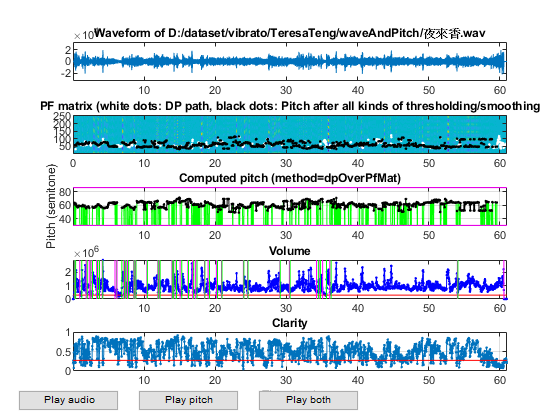
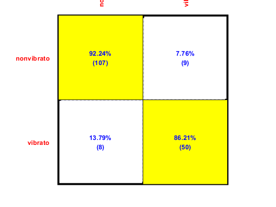
figure;
myTic=tic;
auFile='D:\dataset\vibrato\female\combined-female.wav';
wObj=hmmEval4audio(auFile, vdOpt, vdHmmModel, 1);
fprintf('time=%g sec\n', toc(myTic));
Accuracy=90.2299%
time=7.74257 sec
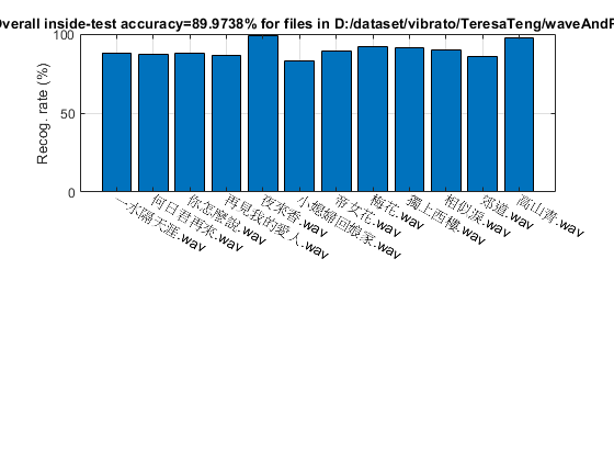
Performance evaluation of HMM via LOO
To evaluate the performance objectively, we can test the LOO accuracy by using "leave-one-file-out":
myTic=tic;
showPlot=1;
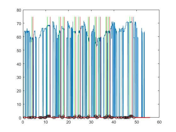
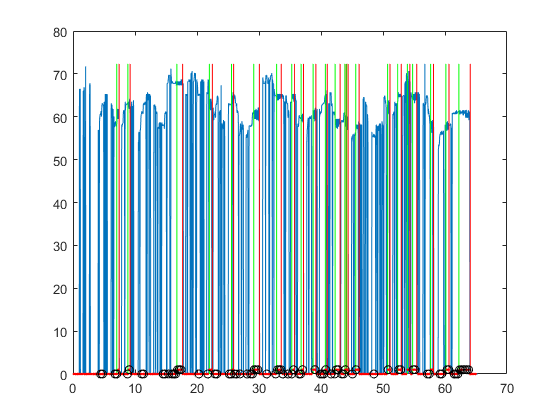
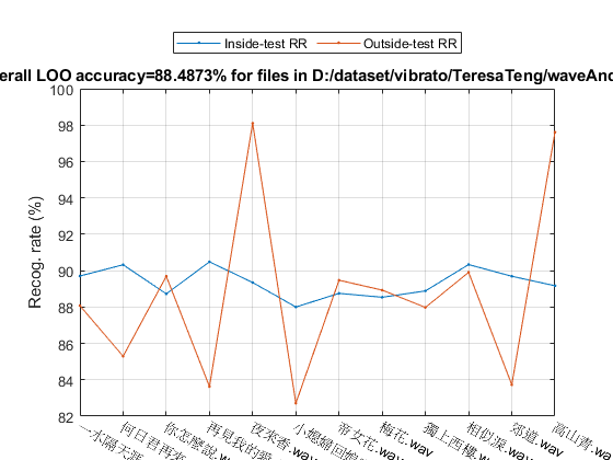
[outsideRr, cvData]=hmmPerfLoo4audio(auSet, vdOpt, showPlot);
fprintf('time=%g sec\n', toc(myTic));
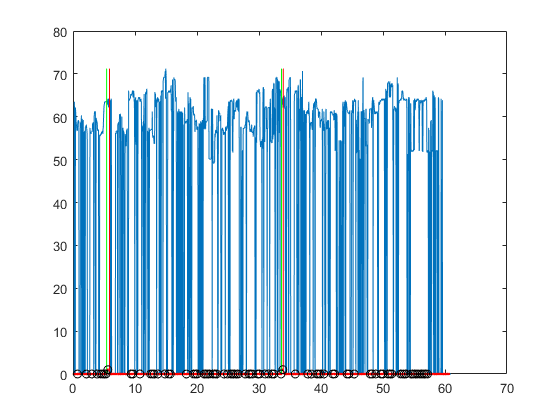
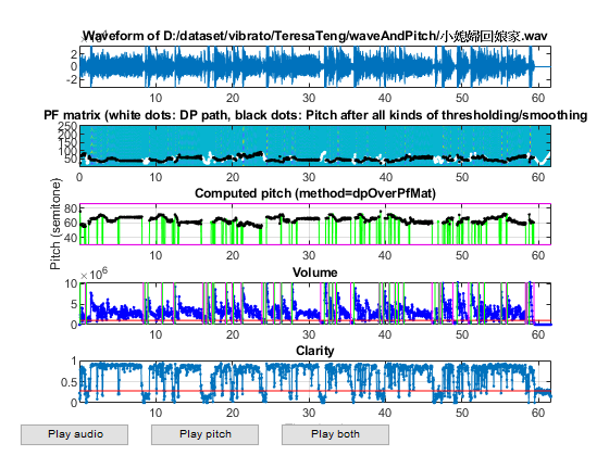
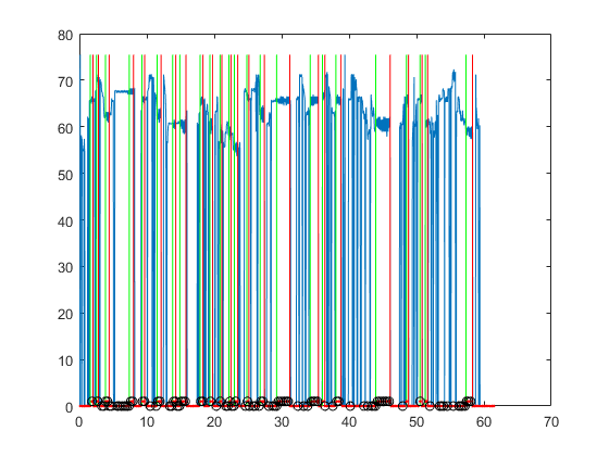
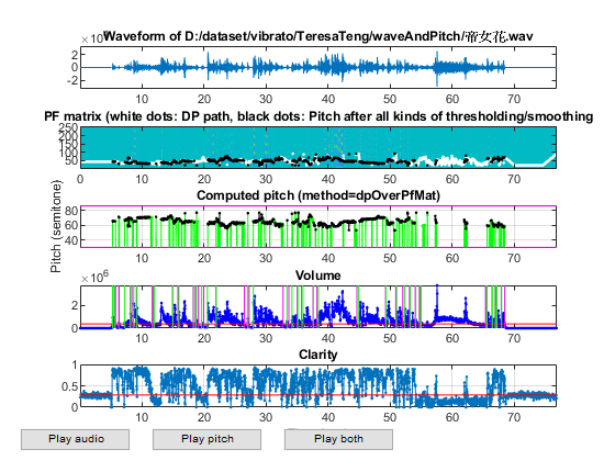
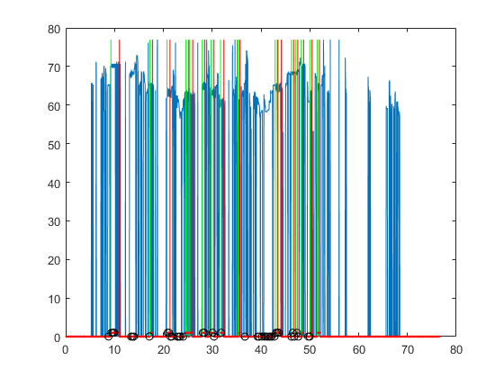
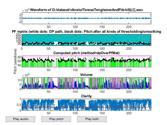
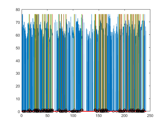
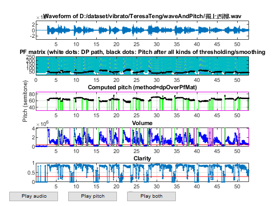
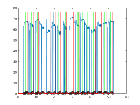
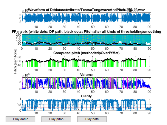
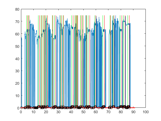
1/12: file=D:\dataset\vibrato\TeresaTeng\waveAndPitch/一水隔天涯.wav
	outsideRr=88.0734%, time=0.35141 sec
2/12: file=D:\dataset\vibrato\TeresaTeng\waveAndPitch/何日君再來.wav
	outsideRr=85.2941%, time=0.21635 sec
3/12: file=D:\dataset\vibrato\TeresaTeng\waveAndPitch/你怎麼說.wav
	outsideRr=89.6907%, time=0.363714 sec
4/12: file=D:\dataset\vibrato\TeresaTeng\waveAndPitch/再見我的愛人.wav
	outsideRr=83.6283%, time=0.298279 sec
5/12: file=D:\dataset\vibrato\TeresaTeng\waveAndPitch/夜來香.wav
	outsideRr=98.1043%, time=0.253 sec
6/12: file=D:\dataset\vibrato\TeresaTeng\waveAndPitch/小媳婦回娘家.wav
	outsideRr=82.7103%, time=0.259102 sec
7/12: file=D:\dataset\vibrato\TeresaTeng\waveAndPitch/帝女花.wav
	outsideRr=89.4737%, time=0.385621 sec
8/12: file=D:\dataset\vibrato\TeresaTeng\waveAndPitch/梅花.wav
	outsideRr=88.9286%, time=0.186022 sec
9/12: file=D:\dataset\vibrato\TeresaTeng\waveAndPitch/獨上西樓.wav
	outsideRr=87.9781%, time=0.3223 sec
10/12: file=D:\dataset\vibrato\TeresaTeng\waveAndPitch/相似淚.wav
	outsideRr=89.9054%, time=0.250629 sec
11/12: file=D:\dataset\vibrato\TeresaTeng\waveAndPitch/郊道.wav
	outsideRr=83.7264%, time=0.175292 sec
12/12: file=D:\dataset\vibrato\TeresaTeng\waveAndPitch/高山青.wav
	outsideRr=97.6077%, time=0.246909 sec
Overall LOO accuracy=88.4873%
time=3.40379 sec
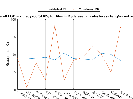
Our previous analysis indicates that input normalization can improve the accuracy. So here we shall try the normalized input for HMM training and test:
myTic=tic;
[~, mu, sigma]=inputNormalize(DS.input);
for i=1:length(auSet)
	auSet(i).feature=inputNormalize(auSet(i).feature, mu, sigma);
end
[outsideRr, cvData]=hmmPerfLoo4audio(auSet, vdOpt, 1);
fprintf('time=%g sec\n', toc(myTic));
1/12: file=D:\dataset\vibrato\TeresaTeng\waveAndPitch/一水隔天涯.wav
	outsideRr=88.9908%, time=0.337122 sec
2/12: file=D:\dataset\vibrato\TeresaTeng\waveAndPitch/何日君再來.wav
	outsideRr=80.6723%, time=0.204561 sec
3/12: file=D:\dataset\vibrato\TeresaTeng\waveAndPitch/你怎麼說.wav
	outsideRr=87.6289%, time=0.380082 sec
4/12: file=D:\dataset\vibrato\TeresaTeng\waveAndPitch/再見我的愛人.wav
	outsideRr=82.7434%, time=0.248367 sec
5/12: file=D:\dataset\vibrato\TeresaTeng\waveAndPitch/夜來香.wav
	outsideRr=98.1043%, time=0.220155 sec
6/12: file=D:\dataset\vibrato\TeresaTeng\waveAndPitch/小媳婦回娘家.wav
	outsideRr=82.7103%, time=0.207711 sec
7/12: file=D:\dataset\vibrato\TeresaTeng\waveAndPitch/帝女花.wav
	outsideRr=88.3459%, time=0.391308 sec
8/12: file=D:\dataset\vibrato\TeresaTeng\waveAndPitch/梅花.wav
	outsideRr=89.0476%, time=0.186448 sec
9/12: file=D:\dataset\vibrato\TeresaTeng\waveAndPitch/獨上西樓.wav
	outsideRr=92.3497%, time=0.353077 sec
10/12: file=D:\dataset\vibrato\TeresaTeng\waveAndPitch/相似淚.wav
	outsideRr=89.9054%, time=0.252326 sec
11/12: file=D:\dataset\vibrato\TeresaTeng\waveAndPitch/郊道.wav
	outsideRr=84.9057%, time=0.237645 sec
12/12: file=D:\dataset\vibrato\TeresaTeng\waveAndPitch/高山青.wav
	outsideRr=97.6077%, time=0.253238 sec
Overall LOO accuracy=88.3416%
time=3.38385 sec
Summary
This is a brief tutorial on using HMM for vibrato detection. There are several directions for further improvement:
- Investigate new features for VD.
- Change the configuration of the GMM used in HMM.
- Use of other classifiers for VD.
Appendix
List of functions, scripts, and datasets used in this script:
Date and time when finishing this script:
fprintf('Date & time: %s\n', char(datetime));
Date & time: 18-Jan-2020 19:51:34
Overall elapsed time:
toc(scriptStartTime)
Elapsed time is 276.781630 seconds.
Jyh-Shing Roger Jang, created on
datetime
ans =

  datetime

   18-Jan-2020 19:51:34
If you are interested in the original MATLAB code for this page, you can type "grabcode(URL)" under MATLAB, where URL is the web address of this page.