Tutorial on music genre classification

This tutorial explains the basics of music genre classification (MGC) using MFCC (mel-frequency cepstral coefficients) as the features for classification. The dataset used here is GTZAN dataseet.

Contents

Preprocessing

Before we start, let's add necessary toolboxes to the search path of MATLAB:

addpath d:/users/jang/matlab/toolbox/utility
addpath d:/users/jang/matlab/toolbox/sap
addpath d:/users/jang/matlab/toolbox/machineLearning
addpath d:/users/jang/matlab/toolbox/machineLearning/externalTool/libsvm-3.21/matlab	% For using SVM classifier

All the above toolboxes can be downloaded from the author's toolbox page. Make sure you are using the latest toolboxes to work with this script.

For compatibility, here we list the platform and MATLAB version that we used to run this script:

fprintf('Platform: %s\n', computer);
fprintf('MATLAB version: %s\n', version);
fprintf('Script starts at %s\n', char(datetime));
scriptStartTime=tic;	% Timing for the whole script

Platform: PCWIN64
MATLAB version: 8.5.0.197613 (R2015a)
Script starts at 04-Feb-2017 20:33:17

Dataset collection

First of all, we shall collect all the audio files from the corpus directory. Note that

auDir='d:/dataSet/musicGenreClassification/GTZAN';
opt=mmDataCollect('defaultOpt');
opt.extName='au';
auSet=mmDataCollect(auDir, opt, 1);

Collecting 1000 files with extension "au" from "d:/dataSet/musicGenreClassification/GTZAN"...

Feature extraction

For each audio, we need to extract the corresponding feature vector for classification. We shall use the function mgcFeaExtract.m (which MFCC and its statistics) for feature extraction. We also need to put all the dataset into a single variable "ds" which is easier for further processing, including classifier construction and evaluation.

if ~exist('ds.mat', 'file')
	myTic=tic;
	opt=dsCreateFromMm('defaultOpt');
	opt.auFeaFcn=@mgcFeaExtract;	% Function for feature extraction
	opt.auFeaOpt=feval(opt.auFeaFcn, 'defaultOpt');	% Feature options
	opt.auEpdFcn='';		% No need to do endpoint detection
	ds=dsCreateFromMm(auSet, opt, 1);
	fprintf('Time for feature extraction over %d files = %g sec\n', length(auSet), toc(myTic));
	fprintf('Saving ds.mat...\n');
	save ds ds
else
	fprintf('Loading ds.mat...\n');
	load ds.mat
end

Loading ds.mat...

Note that if feature extraction is lengthy, we can simply load ds.mat which has been save in the above code snippet.

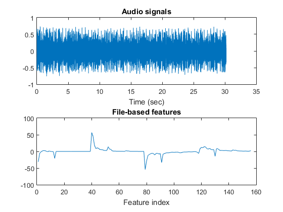
Basically the extracted features are based on MFCC's statistics, including mean, std, min, and max along each dimension. Since MFCC has 39 dimensions, the extracted file-based features has 156 (= 39*4) dimensions. You can type try "mgcFeaExtract" on one of the audio file to plot the result:

auFile=[auDir, '/disco/disco.00001.au'];
figure; mgcFeaExtract(auFile, [], 1);

Dataset visualization

Once we have every piece of necessary information stored in "ds", we can invoke many different functions in Machine Learning Toolbox for data visualization and classification.

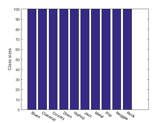
For instance, we can display the size of each class:

figure;
[classSize, classLabel]=dsClassSize(ds, 1);

156 features
1000 instances
10 classes

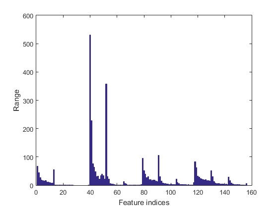
We can plot the range of features of the dataset:

figure; dsRangePlot(ds);

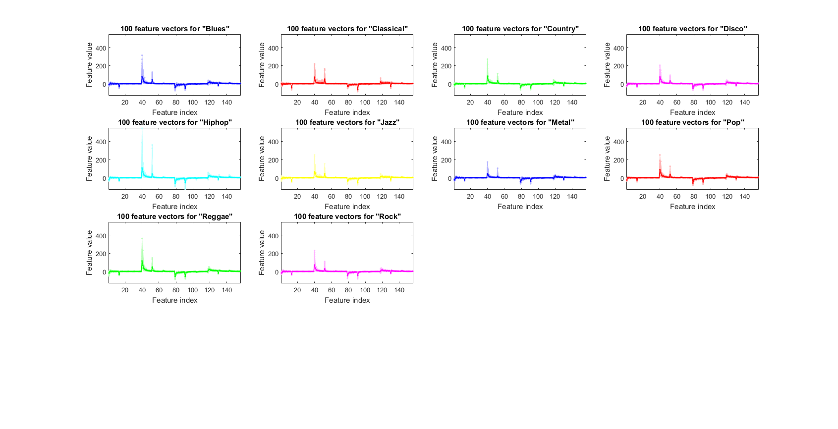
We can plot the feature vectors within each class:

figure; dsFeaVecPlot(ds); figEnlarge;

Dimensionality reduction

The dimension of the feature vector is quite large:

dim=size(ds.input, 1);
fprintf('Feature dimensions = %d\n', dim);

Feature dimensions = 156

We shall consider dimensionality reduction via PCA (principal component analysis). First, let's plot the cumulative variance given the descending eigenvalues of PCA:

[input2, eigVec, eigValue]=pca(ds.input);
cumVar=cumsum(eigValue);
cumVarPercent=cumVar/cumVar(end)*100;
figure; plot(cumVarPercent, '.-');
xlabel('No. of eigenvalues');
ylabel('Cumulated variance percentage (%)');
title('Variance percentage vs. no. of eigenvalues');

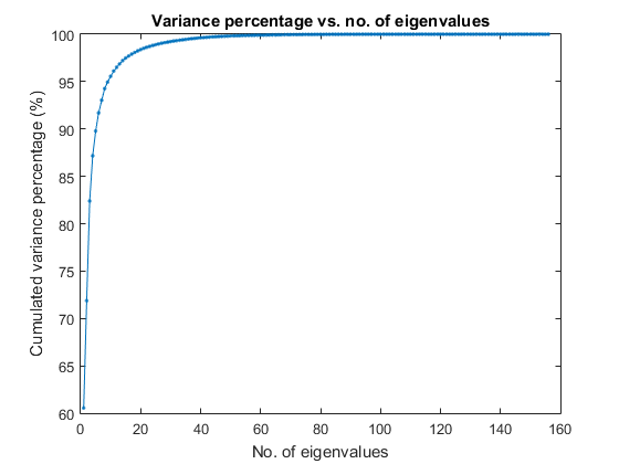
A reasonable choice is to retain the dimensionality such that the cumulative variance percentage is larger than a threshold, say, 95%, as follows:

cumVarTh=95;
index=find(cumVarPercent>cumVarTh);
newDim=index(1);
ds2=ds;
ds2.input=input2(1:newDim, :);
fprintf('Reduce the dimensionality to %d to keep %g%% cumulative variance via PCA.\n', newDim, cumVarTh);

Reduce the dimensionality to 10 to keep 95% cumulative variance via PCA.

However, our experiment indicates that if we use PCA for dimensionality reduction, the accuracy will be lower. As a result, we shall keep all the features for further exploration.

In order to visualize the distribution of the dataset, we can project the original dataset into 2-D space. This can be achieved by LDA (linear discriminant analysis):

ds2d=lda(ds);
ds2d.input=ds2d.input(1:2, :);
figure; dsScatterPlot(ds2d); xlabel('Input 1'); ylabel('Input 2');
title('Features projected on the first 2 lda vectors');

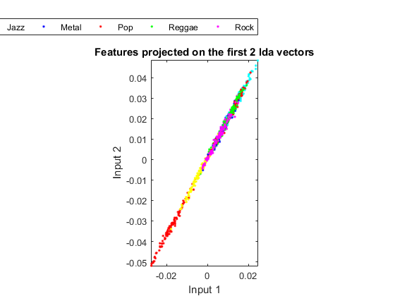
Apparently the separation among classes is not obvious. This indicates that either the features or LDA are not very effective.

Classification

We can try the most straightforward KNNC (k-nearest neighbor classifier):

[rr, ~]=knncLoo(ds);
fprintf('rr=%g%% for original ds\n', rr*100);
ds2=ds; ds2.input=inputNormalize(ds2.input);
[rr2, computed]=knncLoo(ds2);
fprintf('rr=%g%% for ds after input normalization\n', rr2*100);

rr=57.6% for original ds
rr=64.9% for ds after input normalization

Again, the vanilla KNNC does not give satisfactory result. So we shall try other potentially better classifiers, such as SVM. Before try SVM, here we use a function mgcOptSet.m to put all the MGC-related options in a single file. This will be easier for us to change a single option in this file and check out the accuracy of MGC. Here is the code for using SVM:

myTic=tic;
mgcOpt=mgcOptSet;
if mgcOpt.useInputNormalize, ds.input=inputNormalize(ds.input);	end		% Input normalization
cvPrm=crossValidate('defaultOpt');
cvPrm.foldNum=mgcOpt.foldNum;
cvPrm.classifier=mgcOpt.classifier;
plotOpt=1;
figure; [tRrMean, vRrMean, tRr, vRr, computedClass]=crossValidate(ds, cvPrm, plotOpt); figEnlarge;
fprintf('Time for cross-validation = %g sec\n', toc(myTic));

Fold = 100/1000
Fold = 200/1000
Fold = 300/1000
Fold = 400/1000
Fold = 500/1000
Fold = 600/1000
Fold = 700/1000
Fold = 800/1000
Fold = 900/1000
Fold = 1000/1000
Training RR=99.01%, Validating RR=77.00%, classifier=svmc, no. of folds=1000
Time for cross-validation = 490.748 sec

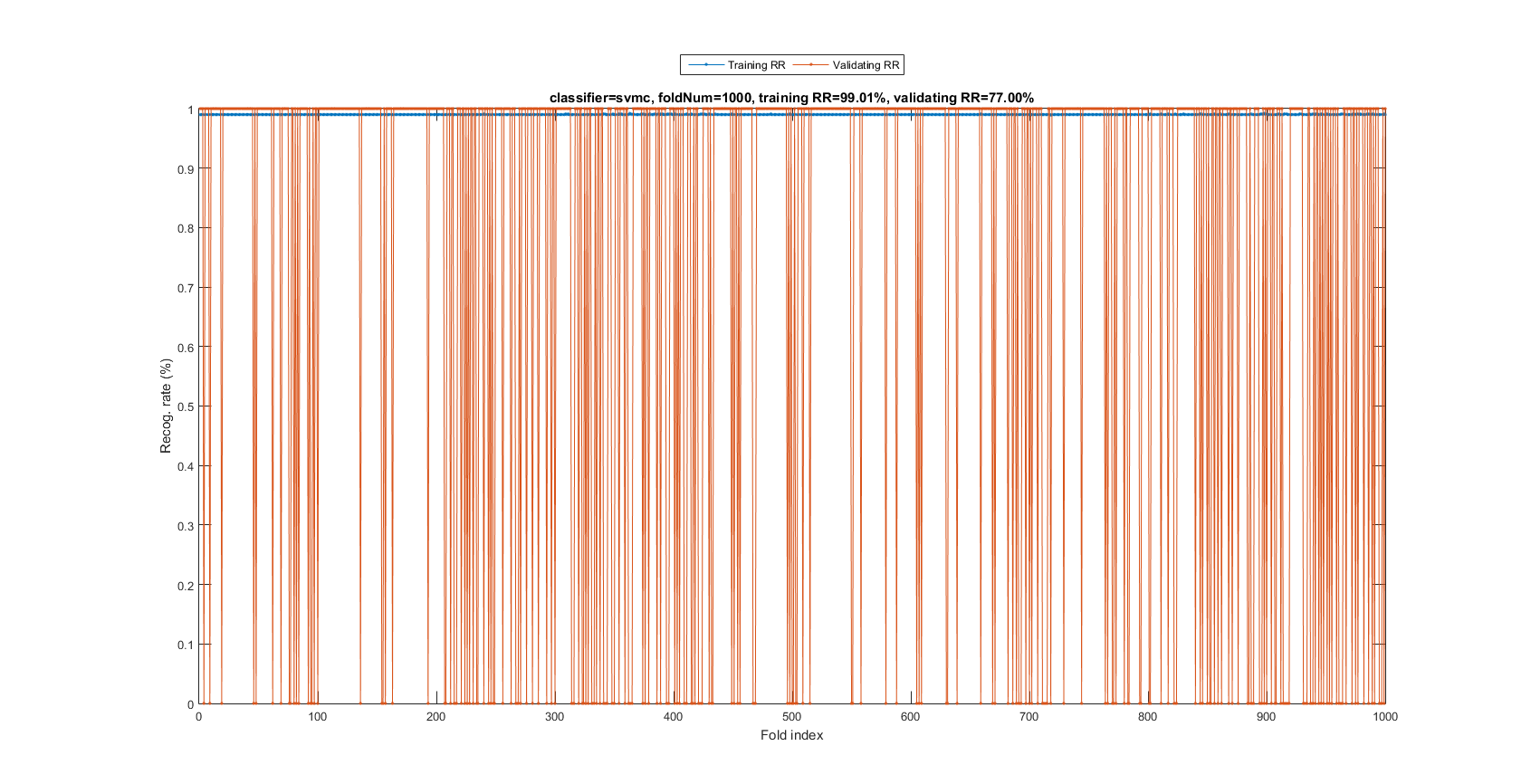
The recognition rate is 77%, indicating SVM is a much more effective classifier.

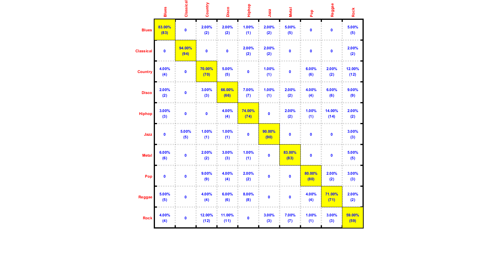
We can plot the confusion matrix:

for i=1:length(computedClass)
	computed(i)=computedClass{i};
end
desired=ds.output;
confMat = confMatGet(desired, computed);
cmOpt=confMatPlot('defaultOpt');
cmOpt.className=ds.outputName;
confMatPlot(confMat, cmOpt); figEnlarge;

Summary

This is a brief tutorial on music genre classification based on MFCC's statistics. There are several directions for further improvement:

Appendix

List of functions and datasets used in this script

Date and time when finishing this script:

fprintf('Date & time: %s\n', char(datetime));

Date & time: 04-Feb-2017 20:41:37

Overall elapsed time:

toc(scriptStartTime)

Elapsed time is 499.976553 seconds.

Jyh-Shing Roger Jang.

Published with MATLAB® R2015a