Tutorial on Beat Assessment for Metronome App.

In this tutorial, we shall explain the basics of beat assessment (or scoring) for software-based metronome.

Contents

Analysis of the pure ticks

Before we start, let's add necessary toolboxes to the search path of MATLAB:

addpath /users/jang/matlab/toolbox/utility
addpath /users/jang/matlab/toolbox/sap
addpath /users/jang/books/audioSignalProcessing/appNote/beatTracking

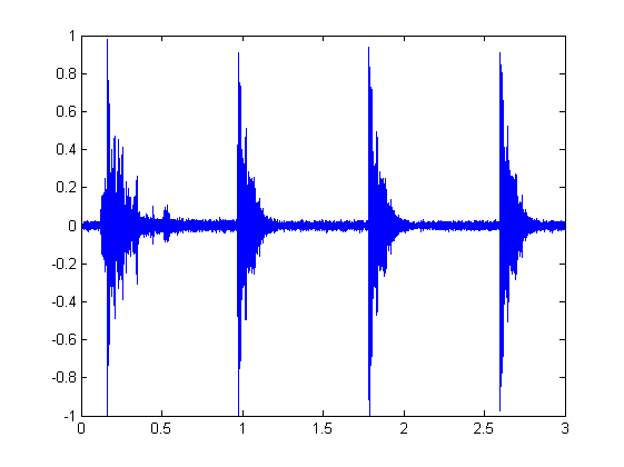
First of all, we can read a recording of piano performance by iPhone/iPad with the sound of ticks coming from a software metronome. We assume that the first 4 ticks (occurring in the first 3 seconds) are clean without any instrument sound.

waveFile='D:\dataSet\metronome\set03_iPod\13_50.wav';
wObj=waveFile2obj(waveFile);
pureTickDuration=3;
cutIndex=pureTickDuration*wObj.fs;
wObj2=wObj; wObj2.signal=wObj2.signal(1:cutIndex);	% wObj2 is pure ticks
plot((1:cutIndex)/wObj2.fs, wObj2.signal);

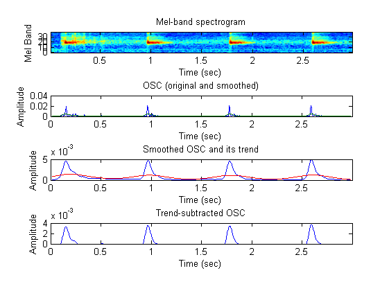
We can then plot the onset detection function (ODF, also known as novelty curve):

btOpt=btOptSet;
[ncObj, rawNc, smoothedNc, localMeanNc, msSpec]=wave2osc(wObj2, btOpt.oscOpt, 1);

Then we perform beat tracking to find the IBI:

btOpt.type='constant';
cBeat=beatTracking(wObj2, btOpt);
ibi=diff(cBeat);
tickPeriod=mean(ibi(2:3));	% Assuming the first tick is not stable

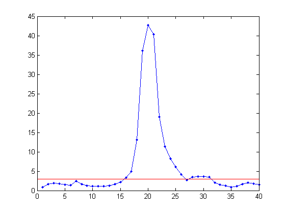
Then we can find the frequency bins not to be used in computing the onset detection function of the music:

sumSpec=sum(msSpec,2);
th=(max(sumSpec)-min(sumSpec))*0.05+min(sumSpec);
figure; plot(sumSpec, '.-');
axisLimit=axis;
line(axisLimit(1:2), th*[1 1], 'color', 'r');
deleteIndex=find(sumSpec>th);

Remove spectral components of the ticks

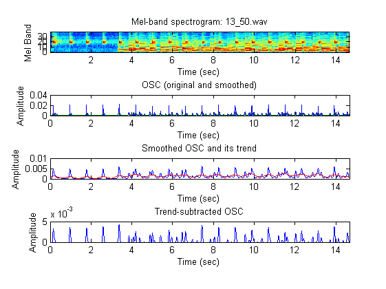
Once the frequency indices not to be used in computing ODF are identified, we can put they back to the computation of ODF:

btOpt.deleteIndex=deleteIndex;
plotOpt=1;
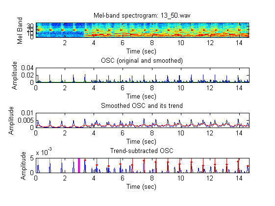
figure; [ncObj, rawNc, smoothedNc, localMeanNc, msSpec]=wave2osc(wObj, btOpt.oscOpt, plotOpt);
[parentDir, mainName]=fileparts(waveFile);
subplot(411), title(sprintf('Mel-band spectrogram: %s.wav', strPurify4label(mainName)));

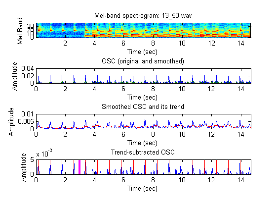
We can then overlay the tick positions to see if they match the onsets. The should be a good criterion for scoring.

subplot(414);
axisLimit=axis;
for i=1:length(cBeat)
	line(cBeat(i)*[1 1], axisLimit(3:4), 'color', 'r');
end
line(cutIndex/wObj.fs*[1 1], axisLimit(3:4), 'color', 'm', 'linewidth', 3);
nextBeatPos=cBeat(end)+tickPeriod;
while nextBeatPos<=(length(wObj.signal)-1)/wObj.fs
	line(nextBeatPos*[1 1], axisLimit(3:4), 'color', 'r');
	nextBeatPos=nextBeatPos+tickPeriod;
end

Function for beat assessment

As shown in the last subplot, if the onsets coincide with the ticks, then the beat assessment should have a high score. Otherwise the score should be low. Therefore we can compute the distance between each tick and its nearest onset. Then we can use the average distance to determine a score between 0 and 100.

Since the above procedure will be used again and again, we have packed the statements into a function beatAssess.m. An example of using the function is shown next:

waveFile='D:\dataSet\metronome\set03_iPod\13_50.wav';
wObj=waveFile2obj(waveFile);
opt=beatAssess('defaultOpt');
showPlot=1;
[score, avgDist]=beatAssess(wObj, opt, showPlot)

score =

   80.3347


avgDist =

    0.0245

Performance evaluation

In general, the average distance should have a high correlation with human's scores (or the so-called groundtruth scores). To verify this, we can invoke the function for a set of recordings with groundtruth scores and show the distribution of distances vs. groundtruth scores:

waveDir='D:\dataSet\metronome\set04';
waveData=recursiveFileList(waveDir, 'wav');
opt=beatAssess('defaultOpt');
showPlot=0;
for i=1:length(waveData)
	file=waveData(i).path;
	[parentDir, mainName]=fileparts(file);
	fprintf('%d/%d: file=%s\n', i, length(waveData), file);
	[score(i), distance(i)]=beatAssess(waveData(i).path, opt, showPlot);
	items=split(mainName, '_');
	gdScore(i)=eval(items{end});
	position{i}=items{3};
	if showPlot, fprintf('Press any key to continue...'); pause; fprintf('\n'); end
end
figure;
plot(distance, gdScore, 'marker', '.', 'markerSize', 40, 'color', 'r', 'linestyle', 'none');
for i=1:length(distance)
	[parentDir, mainName]=fileparts(waveData(i).path);
	textH(i)=text(distance(i), gdScore(i), strPurify4label(['   ', mainName]), 'rot', 270);
end
xlabel('Distance');
ylabel('Groundtruth score');

1/11: file=D:\dataSet\metronome\set04/042701_yuchieh_右側沙發椅_ipodtouch_60.wav
2/11: file=D:\dataSet\metronome\set04/042702_yuchieh_右側沙發椅_ipodtouch_80.wav
3/11: file=D:\dataSet\metronome\set04/042703_yuchieh_右側沙發椅_ipodtouch_90.wav
4/11: file=D:\dataSet\metronome\set04/042704_yuchieh_鋼琴下方木板_ipodtouch_85.wav
5/11: file=D:\dataSet\metronome\set04/042705_yuchieh_鋼琴下方木板_ipodtouch_50.wav
6/11: file=D:\dataSet\metronome\set04/042706_yuchieh_鋼琴下方木板_ipodtouch_10.wav
7/11: file=D:\dataSet\metronome\set04/042707_yuchieh_右側木桌_ipodtouch_95.wav
8/11: file=D:\dataSet\metronome\set04/042708_yuchieh_鋼琴上方_ipodtouch_50.wav
9/11: file=D:\dataSet\metronome\set04/042709_yuchieh_鋼琴上方_ipodtouch_20.wav
10/11: file=D:\dataSet\metronome\set04/042710_yuchieh_鋼琴上方_ipodtouch_90.wav
11/11: file=D:\dataSet\metronome\set04/042711_yuchieh_鋼琴上方_ipodtouch_95.wav

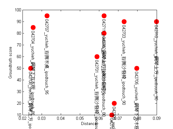
From the distribution, we can see a trend from left-upper to right-lower corners. That is, the higher the distance, the lower the score. This conform to our intuition of scoring. However, we still to spend more time on identify the factors that change the score, and use these factors for better score modeling.

Summary

This is a brief tutorial on beat assessment. There are several directions for further improvement:

Jyh-Shing Roger Jang, 2013/05/01.

Published with MATLAB® 7.12