Tutorial on coin recognition
This tutorial explains the basics of coin recognition based on the sound when the coin is dropped to the ground.
Contents
Preprocessing
Before we start, let's add necessary toolboxes to the search path of MATLAB:
addpath d:/users/jang/matlab/toolbox/utility
addpath d:/users/jang/matlab/toolbox/sap
addpath d:/users/jang/matlab/toolbox/machineLearning
All the above toolboxes can be downloaded from the author's toolbox page. Make sure you are using the latest toolboxes to work with this script.
For compatibility, here we list the platform and MATLAB version that we used to run this script:
fprintf('Platform: %s\n', computer);
fprintf('MATLAB version: %s\n', version);
fprintf('Script starts at %s\n', char(datetime));
scriptStartTime=tic;	% Timing for the whole script
Platform: PCWIN64
MATLAB version: 9.6.0.1214997 (R2019a) Update 6
Script starts at 18-Jan-2020 19:51:43
Dataset collection
First of all, we can collect all the sound files. The dataset can be found at this link. We can use the commmand "mmDataCollect" to collect all the file information:
auDir='coinSound';
opt=mmDataCollect('defaultOpt');
opt.extName='wav';
auSet=mmDataCollect(auDir, opt, 1);
Collecting 20 files with extension "wav" from "coinSound"...
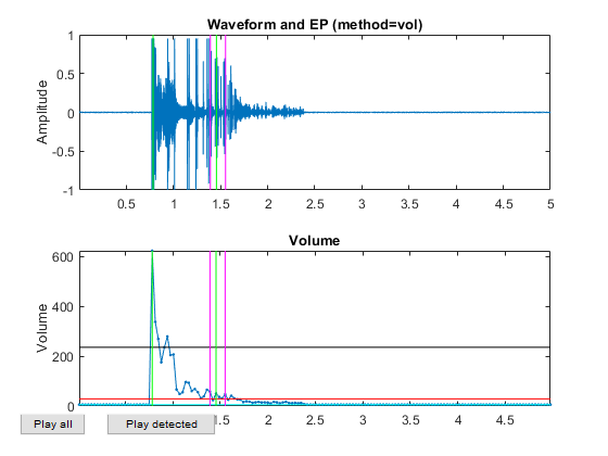
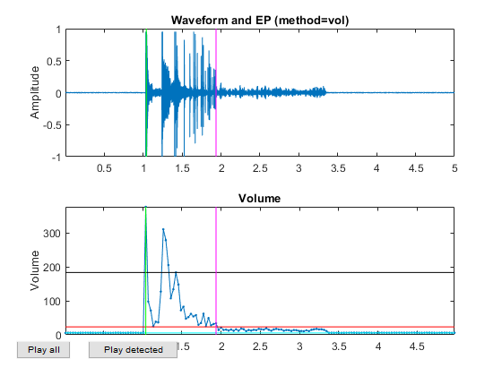
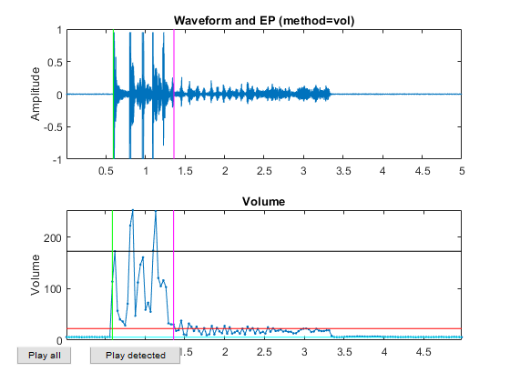
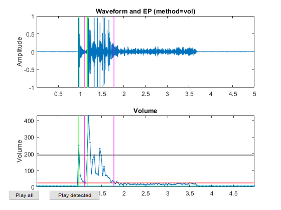
We need to perform feature extraction and put all the dataset into a format that is easier for further processing, including classifier construction and evaluation.
myTic=tic;
%if ~exist('ds.mat', 'file')
	opt=dsCreateFromMm('defaultOpt');
	opt.auFeaFcn=@auFeaMfcc;		% Function for feature extraction
	opt.auEpdOpt.method='vol';
	%opt.auEpdOpt.volRatio=0.02;	% To have the right EPD, but it doesn't help recognition!
	ds=dsCreateFromMm(auSet, opt);
	fprintf('Saving ds.mat...\n'); save ds ds
%else
%	fprintf('Loading ds.mat...\n'); load ds.mat
%end
fprintf('time=%g sec\n', toc(myTic));
Extracting features from each multimedia object...
2/20: file=coinSound/01/1nt_2.wav, time=0.217342 sec
4/20: file=coinSound/01/1nt_4.wav, time=0.243223 sec
6/20: file=coinSound/05/5nt_1.wav, time=0.224709 sec
8/20: file=coinSound/05/5nt_3.wav, time=0.211857 sec
10/20: file=coinSound/05/5nt_5.wav, time=0.217799 sec
12/20: file=coinSound/10/10nt_2.wav, time=0.213291 sec
14/20: file=coinSound/10/10nt_4.wav, time=0.220368 sec
16/20: file=coinSound/50/50nt_1.wav, time=0.219181 sec
18/20: file=coinSound/50/50nt_3.wav, time=0.213423 sec
20/20: file=coinSound/50/50nt_5.wav, time=0.221815 sec
Saving ds.mat...
time=4.52943 sec
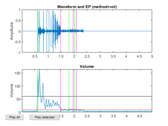
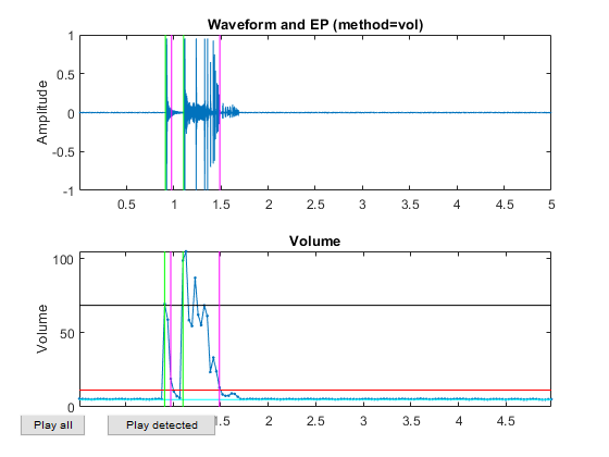
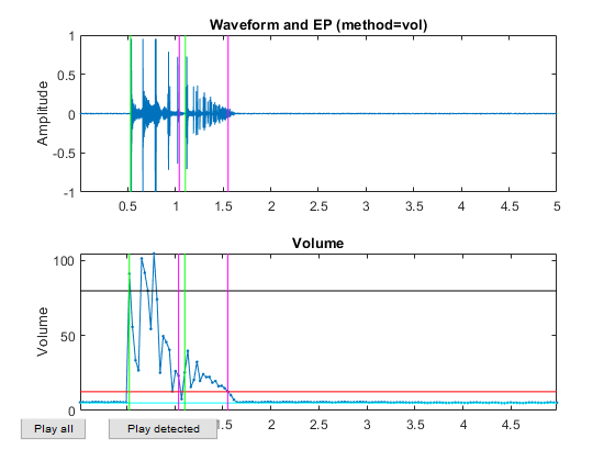
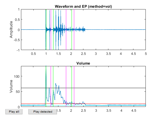
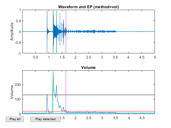
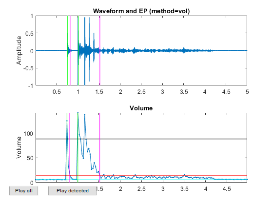
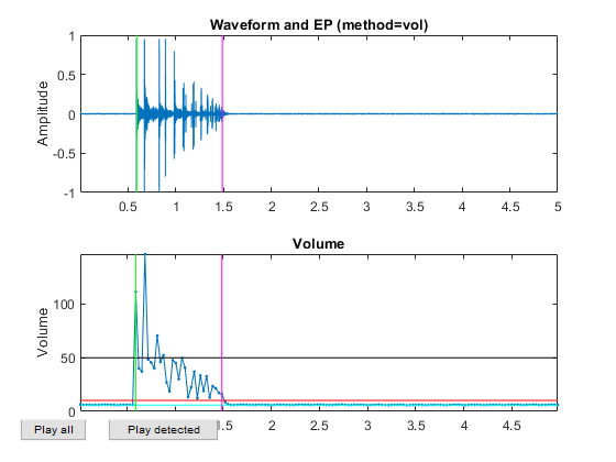
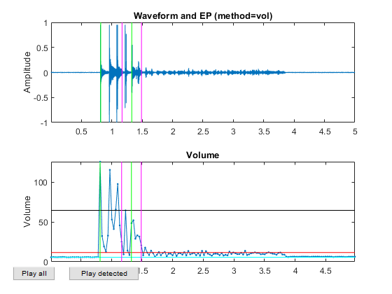
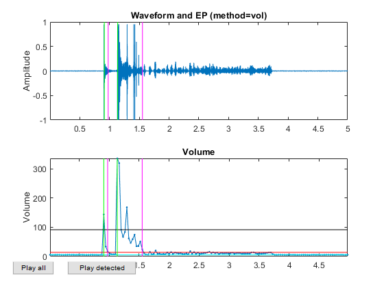
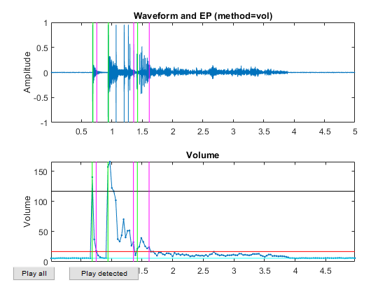
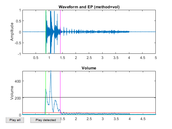
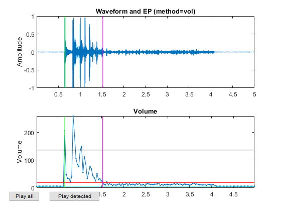
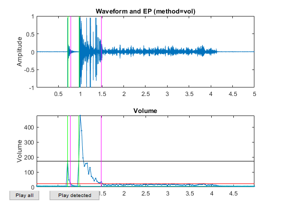
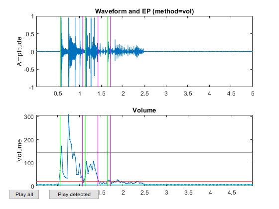
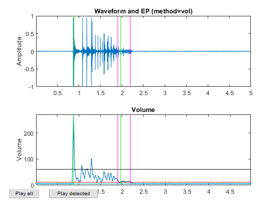
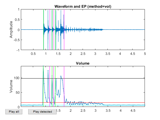
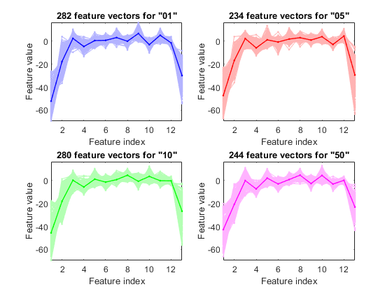
Now all the frame-based features are extracted and stored in "ds". Next we can try to plot the extracted features for each class:
figure; dsFeaVecPlot(ds);
Performance evaluation
Now we want to do performance evaluation on LOFOCV (leave-one-file-out cross validation), where each file is a recording of a complete sound event. LOFOCV is proceeded as follows:
opt=perfLoo4audio('defaultOpt');
[ds2, fileRr, frameRr]=perfLoo4audio(ds, opt);
fprintf('Frame-based leave-one-file-out RR=%g%%\n', frameRr*100);
fprintf('File-based leave-one-file-out RR=%g%%\n', fileRr*100);
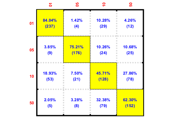
1/20: LOFO for "coinSound/01/1nt_1.wav", time=0.147367 sec
2/20: LOFO for "coinSound/01/1nt_2.wav", time=0.145159 sec
3/20: LOFO for "coinSound/01/1nt_3.wav", time=0.142272 sec
4/20: LOFO for "coinSound/01/1nt_4.wav", time=0.135314 sec
5/20: LOFO for "coinSound/01/1nt_5.wav", time=0.140786 sec
6/20: LOFO for "coinSound/05/5nt_1.wav", time=0.186218 sec
7/20: LOFO for "coinSound/05/5nt_2.wav", time=0.164839 sec
8/20: LOFO for "coinSound/05/5nt_3.wav", time=0.128897 sec
9/20: LOFO for "coinSound/05/5nt_4.wav", time=0.128366 sec
10/20: LOFO for "coinSound/05/5nt_5.wav", time=0.136987 sec
11/20: LOFO for "coinSound/10/10nt_1.wav", time=0.155006 sec
12/20: LOFO for "coinSound/10/10nt_2.wav", time=0.131629 sec
13/20: LOFO for "coinSound/10/10nt_3.wav", time=0.137514 sec
14/20: LOFO for "coinSound/10/10nt_4.wav", time=0.150389 sec
15/20: LOFO for "coinSound/10/10nt_5.wav", time=0.142683 sec
16/20: LOFO for "coinSound/50/50nt_1.wav", time=0.126877 sec
17/20: LOFO for "coinSound/50/50nt_2.wav", time=0.131085 sec
18/20: LOFO for "coinSound/50/50nt_3.wav", time=0.150031 sec
19/20: LOFO for "coinSound/50/50nt_4.wav", time=0.134259 sec
20/20: LOFO for "coinSound/50/50nt_5.wav", time=0.126844 sec
Frame-based leave-one-file-out RR=66.6346%
File-based leave-one-file-out RR=95%
We can plot the frame-based confusion matrix:
confMat=confMatGet(ds2.output, ds2.frameClassIdPredicted);
confOpt=confMatPlot('defaultOpt');
confOpt.className=ds.outputName;
figure; confMatPlot(confMat, confOpt);
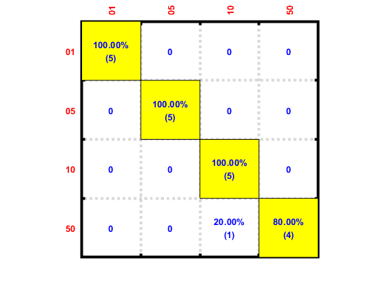
We can also plot the file-based confusion matrix:
confMat=confMatGet(ds2.fileClassId, ds2.fileClassIdPredicted);
confOpt=confMatPlot('defaultOpt');
confOpt.className=ds.outputName;
figure; confMatPlot(confMat, confOpt);
We can also list all the misclassified sounds in a table:
for i=1:length(auSet)
	auSet(i).classPredicted=ds.outputName{ds2.fileClassIdPredicted(i)};
end
mmDataList(auSet);
| Index\Field | File | GT ==> Predicted | Hit | url |
|---|---|---|---|---|
| 1 | 50nt_1.wav | 50 ==> 10 | false | /jang/books/audioSignalProcessing/appNote/coinType/coinSound/50/50nt_1.wav |
Dimensionality reduction
In order to visualize the distribution of the dataset, we need to project the original dataset into 2-D space. This can be achieved by LDA (linear discriminant analysis):
ds2d=lda(ds);
ds2d.input=ds2d.input(1:2, :);
figure; dsScatterPlot(ds2d); xlabel('Input 1'); ylabel('Input 2');
title('MFCC projected on the first 2 lda vectors');
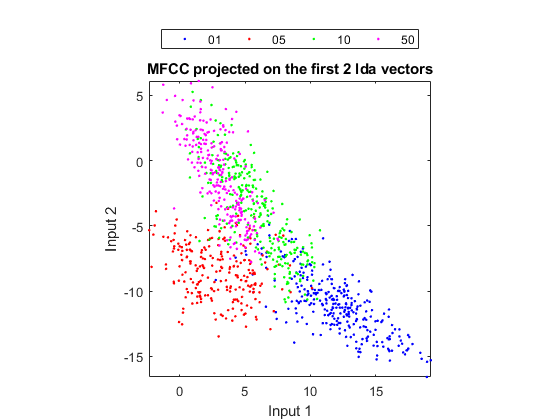
As can be seen from the scatter plot, the overlap between "10" and "50" is the largest among all class pairs, indicating that these two classes are likely to be confused with each other. This is also verified by the confusion matrices shown earlier.
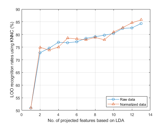
Actually it is possible to do LDA projection and obtain the corresponding accuracies vs. dimensionalities via leave-one-out cross validation over KNNC:
opt=ldaPerfViaKnncLoo('defaultOpt');
opt.mode='exact';
recogRate1=ldaPerfViaKnncLoo(ds, opt);
ds2=ds; ds2.input=inputNormalize(ds2.input);	% input normalization
recogRate2=ldaPerfViaKnncLoo(ds2, opt);
[featureNum, dataNum] = size(ds.input);
plot(1:featureNum, 100*recogRate1, 'o-', 1:featureNum, 100*recogRate2, '^-'); grid on
legend('Raw data', 'Normalized data', 'location', 'southeast');
xlabel('No. of projected features based on LDA');
ylabel('LOO recognition rates using KNNC (%)');
We can also perform input selection to reduce dimensionality:
myTic=tic;
z=inputSelectSequential(ds, inf, [], [], 1); figEnlarge;
toc(myTic)
Construct 91 "" models, each with up to 13 inputs selected from all 13 inputs...

Selecting input 1:
Model 1/91: selected={ 1} => Recog. rate = 33.2%
Model 2/91: selected={ 2} => Recog. rate = 25.8%
Model 3/91: selected={ 3} => Recog. rate = 32.3%
Model 4/91: selected={ 4} => Recog. rate = 34.9%
Model 5/91: selected={ 5} => Recog. rate = 28.2%
Model 6/91: selected={ 6} => Recog. rate = 39.1%
Model 7/91: selected={ 7} => Recog. rate = 37.5%
Model 8/91: selected={ 8} => Recog. rate = 44.0%
Model 9/91: selected={ 9} => Recog. rate = 51.2%
Model 10/91: selected={10} => Recog. rate = 49.0%
Model 11/91: selected={11} => Recog. rate = 55.3%
Model 12/91: selected={12} => Recog. rate = 53.1%
Model 13/91: selected={13} => Recog. rate = 31.9%
Currently selected inputs: 11 => Recog. rate = 55.3%

Selecting input 2:
Model 14/91: selected={11,  1} => Recog. rate = 57.5%
Model 15/91: selected={11,  2} => Recog. rate = 59.9%
Model 16/91: selected={11,  3} => Recog. rate = 56.8%
Model 17/91: selected={11,  4} => Recog. rate = 57.5%
Model 18/91: selected={11,  5} => Recog. rate = 55.3%
Model 19/91: selected={11,  6} => Recog. rate = 59.9%
Model 20/91: selected={11,  7} => Recog. rate = 56.3%
Model 21/91: selected={11,  8} => Recog. rate = 62.5%
Model 22/91: selected={11,  9} => Recog. rate = 65.6%
Model 23/91: selected={11, 10} => Recog. rate = 60.2%
Model 24/91: selected={11, 12} => Recog. rate = 71.1%
Model 25/91: selected={11, 13} => Recog. rate = 57.1%
Currently selected inputs: 11, 12 => Recog. rate = 71.1%

Selecting input 3:
Model 26/91: selected={11, 12,  1} => Recog. rate = 72.1%
Model 27/91: selected={11, 12,  2} => Recog. rate = 74.7%
Model 28/91: selected={11, 12,  3} => Recog. rate = 73.0%
Model 29/91: selected={11, 12,  4} => Recog. rate = 69.8%
Model 30/91: selected={11, 12,  5} => Recog. rate = 72.3%
Model 31/91: selected={11, 12,  6} => Recog. rate = 74.9%
Model 32/91: selected={11, 12,  7} => Recog. rate = 72.2%
Model 33/91: selected={11, 12,  8} => Recog. rate = 73.1%
Model 34/91: selected={11, 12,  9} => Recog. rate = 74.3%
Model 35/91: selected={11, 12, 10} => Recog. rate = 76.4%
Model 36/91: selected={11, 12, 13} => Recog. rate = 72.3%
Currently selected inputs: 11, 12, 10 => Recog. rate = 76.4%

Selecting input 4:
Model 37/91: selected={11, 12, 10,  1} => Recog. rate = 77.7%
Model 38/91: selected={11, 12, 10,  2} => Recog. rate = 78.0%
Model 39/91: selected={11, 12, 10,  3} => Recog. rate = 77.2%
Model 40/91: selected={11, 12, 10,  4} => Recog. rate = 76.3%
Model 41/91: selected={11, 12, 10,  5} => Recog. rate = 75.8%
Model 42/91: selected={11, 12, 10,  6} => Recog. rate = 77.5%
Model 43/91: selected={11, 12, 10,  7} => Recog. rate = 77.2%
Model 44/91: selected={11, 12, 10,  8} => Recog. rate = 76.0%
Model 45/91: selected={11, 12, 10,  9} => Recog. rate = 76.9%
Model 46/91: selected={11, 12, 10, 13} => Recog. rate = 76.8%
Currently selected inputs: 11, 12, 10,  2 => Recog. rate = 78.0%

Selecting input 5:
Model 47/91: selected={11, 12, 10,  2,  1} => Recog. rate = 79.1%
Model 48/91: selected={11, 12, 10,  2,  3} => Recog. rate = 79.8%
Model 49/91: selected={11, 12, 10,  2,  4} => Recog. rate = 77.7%
Model 50/91: selected={11, 12, 10,  2,  5} => Recog. rate = 77.6%
Model 51/91: selected={11, 12, 10,  2,  6} => Recog. rate = 79.1%
Model 52/91: selected={11, 12, 10,  2,  7} => Recog. rate = 79.2%
Model 53/91: selected={11, 12, 10,  2,  8} => Recog. rate = 78.2%
Model 54/91: selected={11, 12, 10,  2,  9} => Recog. rate = 77.9%
Model 55/91: selected={11, 12, 10,  2, 13} => Recog. rate = 78.2%
Currently selected inputs: 11, 12, 10,  2,  3 => Recog. rate = 79.8%

Selecting input 6:
Model 56/91: selected={11, 12, 10,  2,  3,  1} => Recog. rate = 80.0%
Model 57/91: selected={11, 12, 10,  2,  3,  4} => Recog. rate = 78.7%
Model 58/91: selected={11, 12, 10,  2,  3,  5} => Recog. rate = 80.5%
Model 59/91: selected={11, 12, 10,  2,  3,  6} => Recog. rate = 80.9%
Model 60/91: selected={11, 12, 10,  2,  3,  7} => Recog. rate = 80.5%
Model 61/91: selected={11, 12, 10,  2,  3,  8} => Recog. rate = 79.9%
Model 62/91: selected={11, 12, 10,  2,  3,  9} => Recog. rate = 79.4%
Model 63/91: selected={11, 12, 10,  2,  3, 13} => Recog. rate = 79.0%
Currently selected inputs: 11, 12, 10,  2,  3,  6 => Recog. rate = 80.9%

Selecting input 7:
Model 64/91: selected={11, 12, 10,  2,  3,  6,  1} => Recog. rate = 81.9%
Model 65/91: selected={11, 12, 10,  2,  3,  6,  4} => Recog. rate = 80.6%
Model 66/91: selected={11, 12, 10,  2,  3,  6,  5} => Recog. rate = 81.0%
Model 67/91: selected={11, 12, 10,  2,  3,  6,  7} => Recog. rate = 81.0%
Model 68/91: selected={11, 12, 10,  2,  3,  6,  8} => Recog. rate = 80.1%
Model 69/91: selected={11, 12, 10,  2,  3,  6,  9} => Recog. rate = 81.0%
Model 70/91: selected={11, 12, 10,  2,  3,  6, 13} => Recog. rate = 81.3%
Currently selected inputs: 11, 12, 10,  2,  3,  6,  1 => Recog. rate = 81.9%

Selecting input 8:
Model 71/91: selected={11, 12, 10,  2,  3,  6,  1,  4} => Recog. rate = 81.6%
Model 72/91: selected={11, 12, 10,  2,  3,  6,  1,  5} => Recog. rate = 82.4%
Model 73/91: selected={11, 12, 10,  2,  3,  6,  1,  7} => Recog. rate = 83.2%
Model 74/91: selected={11, 12, 10,  2,  3,  6,  1,  8} => Recog. rate = 82.0%
Model 75/91: selected={11, 12, 10,  2,  3,  6,  1,  9} => Recog. rate = 82.9%
Model 76/91: selected={11, 12, 10,  2,  3,  6,  1, 13} => Recog. rate = 82.9%
Currently selected inputs: 11, 12, 10,  2,  3,  6,  1,  7 => Recog. rate = 83.2%

Selecting input 9:
Model 77/91: selected={11, 12, 10,  2,  3,  6,  1,  7,  4} => Recog. rate = 82.9%
Model 78/91: selected={11, 12, 10,  2,  3,  6,  1,  7,  5} => Recog. rate = 84.0%
Model 79/91: selected={11, 12, 10,  2,  3,  6,  1,  7,  8} => Recog. rate = 84.3%
Model 80/91: selected={11, 12, 10,  2,  3,  6,  1,  7,  9} => Recog. rate = 82.3%
Model 81/91: selected={11, 12, 10,  2,  3,  6,  1,  7, 13} => Recog. rate = 82.9%
Currently selected inputs: 11, 12, 10,  2,  3,  6,  1,  7,  8 => Recog. rate = 84.3%

Selecting input 10:
Model 82/91: selected={11, 12, 10,  2,  3,  6,  1,  7,  8,  4} => Recog. rate = 84.1%
Model 83/91: selected={11, 12, 10,  2,  3,  6,  1,  7,  8,  5} => Recog. rate = 84.9%
Model 84/91: selected={11, 12, 10,  2,  3,  6,  1,  7,  8,  9} => Recog. rate = 83.9%
Model 85/91: selected={11, 12, 10,  2,  3,  6,  1,  7,  8, 13} => Recog. rate = 83.2%
Currently selected inputs: 11, 12, 10,  2,  3,  6,  1,  7,  8,  5 => Recog. rate = 84.9%

Selecting input 11:
Model 86/91: selected={11, 12, 10,  2,  3,  6,  1,  7,  8,  5,  4} => Recog. rate = 84.3%
Model 87/91: selected={11, 12, 10,  2,  3,  6,  1,  7,  8,  5,  9} => Recog. rate = 85.2%
Model 88/91: selected={11, 12, 10,  2,  3,  6,  1,  7,  8,  5, 13} => Recog. rate = 85.1%
Currently selected inputs: 11, 12, 10,  2,  3,  6,  1,  7,  8,  5,  9 => Recog. rate = 85.2%

Selecting input 12:
Model 89/91: selected={11, 12, 10,  2,  3,  6,  1,  7,  8,  5,  9,  4} => Recog. rate = 83.8%
Model 90/91: selected={11, 12, 10,  2,  3,  6,  1,  7,  8,  5,  9, 13} => Recog. rate = 84.8%
Currently selected inputs: 11, 12, 10,  2,  3,  6,  1,  7,  8,  5,  9, 13 => Recog. rate = 84.8%

Selecting input 13:
Model 91/91: selected={11, 12, 10,  2,  3,  6,  1,  7,  8,  5,  9, 13,  4} => Recog. rate = 84.5%
Currently selected inputs: 11, 12, 10,  2,  3,  6,  1,  7,  8,  5,  9, 13,  4 => Recog. rate = 84.5%

Overall maximal recognition rate = 85.2%.
Selected 11 inputs (out of 13): 11, 12, 10,  2,  3,  6,  1,  7,  8,  5,  9
Elapsed time is 179.272559 seconds.
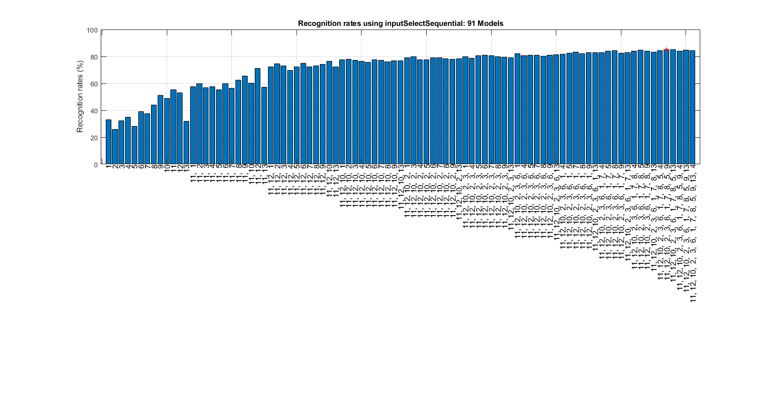
It seems the feature selection is not very effective since the accuracy is the best when all the inputs are selected.
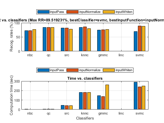
After dimensionality reduction, we can perform all combinations of classifiers and input normalization to search the best performance via leave-one-out cross validation:
myTic=tic;
poOpt=perfCv4classifier('defaultOpt');
poOpt.foldNum=inf;	% Leave-one-out cross validation
figure; [perfData, bestId]=perfCv4classifier(ds, poOpt, 1);
toc(myTic)
structDispInHtml(perfData, 'Performance of various classifiers via cross validation');
Elapsed time is 2016.783502 seconds.
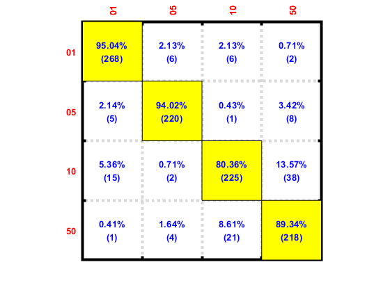
Then we can display the confusion matrix corresponding to the best classifier and the best input normalization scheme:
confMat=confMatGet(ds.output, perfData(bestId).bestComputedClass);
confOpt=confMatPlot('defaultOpt');
confOpt.className=ds.outputName;
figure; confMatPlot(confMat, confOpt);
opt=perfLoo4audio('defaultOpt');
opt.classifier='qc';
opt.classifierOpt=feval([opt.classifier, 'Train'], 'defaultOpt');
[ds2, fileRr, frameRr]=perfLoo4audio(ds, opt);
fprintf('Frame-based leave-one-file-out RR=%g%%\n', frameRr*100);
fprintf('File-based leave-one-file-out RR=%g%%\n', fileRr*100);
1/20: LOFO for "coinSound/01/1nt_1.wav", time=0.0136172 sec
2/20: LOFO for "coinSound/01/1nt_2.wav", time=0.0054627 sec
3/20: LOFO for "coinSound/01/1nt_3.wav", time=0.0066412 sec
4/20: LOFO for "coinSound/01/1nt_4.wav", time=0.0050941 sec
5/20: LOFO for "coinSound/01/1nt_5.wav", time=0.0046561 sec
6/20: LOFO for "coinSound/05/5nt_1.wav", time=0.0060149 sec
7/20: LOFO for "coinSound/05/5nt_2.wav", time=0.0048313 sec
8/20: LOFO for "coinSound/05/5nt_3.wav", time=0.0045429 sec
9/20: LOFO for "coinSound/05/5nt_4.wav", time=0.0062795 sec
10/20: LOFO for "coinSound/05/5nt_5.wav", time=0.0048544 sec
11/20: LOFO for "coinSound/10/10nt_1.wav", time=0.0044577 sec
12/20: LOFO for "coinSound/10/10nt_2.wav", time=0.004715 sec
13/20: LOFO for "coinSound/10/10nt_3.wav", time=0.00472 sec
14/20: LOFO for "coinSound/10/10nt_4.wav", time=0.0047349 sec
15/20: LOFO for "coinSound/10/10nt_5.wav", time=0.0044872 sec
16/20: LOFO for "coinSound/50/50nt_1.wav", time=0.0052304 sec
17/20: LOFO for "coinSound/50/50nt_2.wav", time=0.0046066 sec
18/20: LOFO for "coinSound/50/50nt_3.wav", time=0.0048216 sec
19/20: LOFO for "coinSound/50/50nt_4.wav", time=0.0052425 sec
20/20: LOFO for "coinSound/50/50nt_5.wav", time=0.0050812 sec
Frame-based leave-one-file-out RR=67.6923%
File-based leave-one-file-out RR=90%
Summary
This is a brief tutorial which uses the basic techniques in pattern recognition. There are several directions for further improvement:
- Explore other features (such as magnitude spectrum)
- Verify that endpoint detection has been performed correctly on each recording
- Use other classifiers
Appendix
List of functions and datasets used in this script
Date and time when finishing this script:
fprintf('Date & time: %s\n', char(datetime));
Date & time: 18-Jan-2020 20:28:58
Overall elapsed time:
toc(scriptStartTime)
Elapsed time is 2235.636744 seconds.